Synthetic Galaxies with GANs

The field of deep learning is incredibly broad. Neural networks have found applications in a variety of contexts across myriad disciplines, from classification to clustering to forecasting and beyond. It’s all well and good to analyse data, but can we do the reverse? Is it possible to synthesise new data that is indistinguishable from the original data? This is the principle behind the field of generative deep learning, which in recent years has seen an explosion in activity, with shining examples including DALL-E and its successors/open-source derivatives, models that can generate pictures based solely on a provided caption (or more specifically a prompt). Of course, it’s not just generative art; there exist models capable of composing music, writing essays and even writing code.

Generative deep learning – insofar as its current face today – took off in 2015 with the development of generative adversarial networks (GANs). In this post, I’ll briefly discuss the principles and intuitions behind GANs, before showing how a GAN can be used to generate artificial images of galaxies based on the Galaxy10 DECals dataset.

Learning to Learn

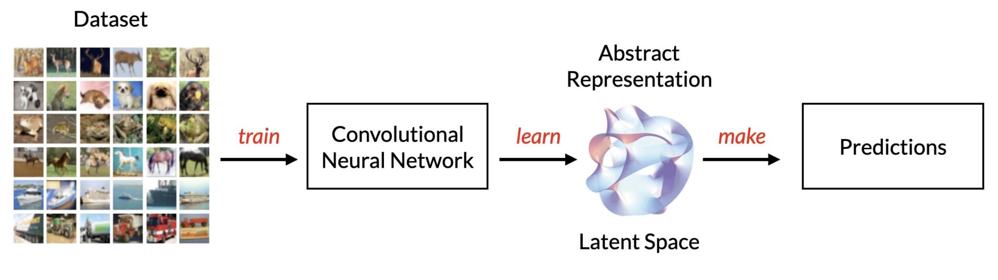
It’s worth taking a step back to look at what it means for a deep learning model – or indeed any AI model – to learn. Suppose we want to train a deep learning model to classify images into various different categories. To train such a model from scratch, we must first provide a training dataset. Usually this includes two components: the actual images themselves, as well as labels that signify which class each image belongs to (or more practically, what the output of the model should be for each image). This type of training with labels is known as supervised learning: each input has a known output. The model is trained to correctly classify each image based on their class by minimising the loss (statistical distance) of its output with respect to the known outputs. Of course, the world isn’t awash with known outputs. How do we ensure that the model is capable of correctly classifying images that it hasn’t seen before? The key to this lies in the model’s ability to generalise, which is all to do with approximating a manifold.

The manifold hypothesis (or manifold assumption) is the idea that all data can be compressed into points on a smooth, differentiable manifold in some arbitrary, lower-dimensional latent space. When we’re training a deep learning model, we’re training it to approximate such a manifold. You can think of the training data merely as a bunch of points that sit somewhere on the manifold, and it is the model’s job to approximate the manifold as closely as possible. This allows the model to analyse data it has never seen before by interpolating along the learned manifold.

It’s important to note that the manifold is merely an abstract representation of the data, the quality of which depends on many factors including the type of model as well as the model’s architecture (which enforces a prior on the nature / “shape” of the data), the training algorithm and choice of optimiser, and, of course, the training data itself. The success of deep learning lies in the ability for models such as convolutional neural networks to compress arbitrary data into these abstract latent spaces, and to henceforth learn meaningful representations of the natural distribution of said data.

Something from Nothing

Perhaps you can see where this is going. In order to actually do anything useful with deep learning, we must first train a model to learn an abstract representation of some training data. Convolutional neural networks do this through applying many convolutional layers in order to extract progressively more abstract features. An input image is, for the most part, ultimately processed down into a vector (the penultimate Dense layer right before the output layer, for instance). Now, what if we turned this process around? (Or, as the line in Ex Machina goes, “reverse the challenge”). What if, instead of starting with an image and obtaining a vector, we start with a vector and use this to generate an image?

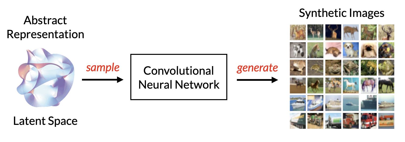
Our goal is thus to come up with a generative model: a probabilistic model that approximates the distribution that underlies some arbitrary training data, so that it can then sample from this distribution to generate new data. The relatively nascent field of generative deep learning seeks to leverage the power of neural networks to create advanced generative models, capable of everything from art, to synthesising speech, to composing music and even to write code. All of this is made possible by the manifold hypothesis, and the ability for CNNs to compress data into a latent space.

Zero-Sum Games

So, how do we learn such a latent space and, subsequently, generate new data? One method is to first encode some data into a latent space, then decode random points from that latent space back into the original data (this is the method behind autoencoders). Another method is to train a generative adversarial network. GANs actually consist of two separate neural networks that are trained in tandem.

• A generator, which takes a vector (corresponding to a point that has been randomly sampled in some latent space) as its input, and outputs an image.
• The discriminator, which takes an image as its input, and must correctly determine whether the image is real (i.e. from the training data), or whether it is a fake image synthesised by the generator.

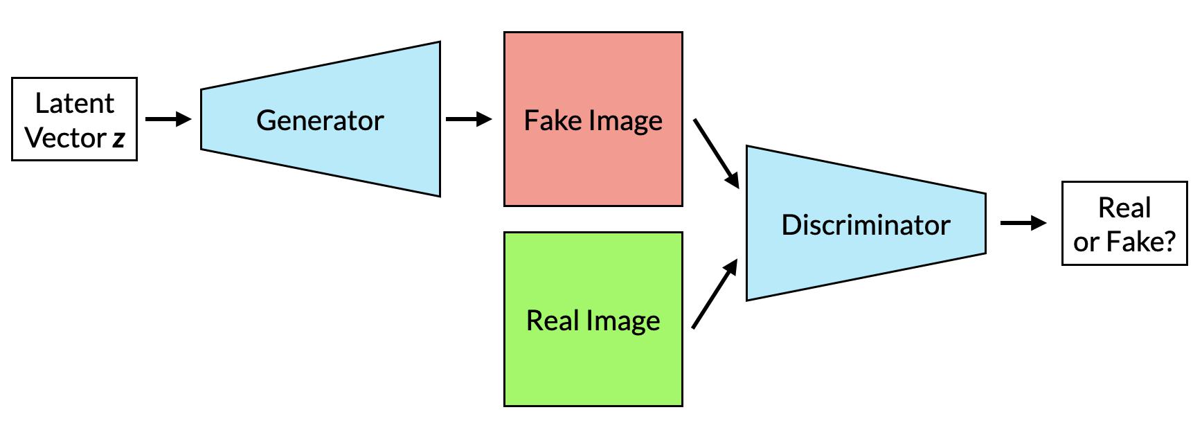
The goal here is for the generator to “fool” the discriminator into thinking its images are real. At the same time, however, the discriminator is learning to correctly distinguish the fake images from the real ones. As the discriminator improves, so too must the generator improve. GANs are thus inherently dynamic; the generator and discriminator are two players in a zero-sum game, each trying to outdo the other. The ultimate goal of training is thus not to seek a global minimum (or maximum) but instead an equilibrium (ideally this ought to be the Nash equilibrium, although recent studies have suggested that GANs may not have Nash equilibria). We can see this by inspecting the loss function, which in this case is a type of minimax loss: \[ \min_{G}\max_{D} V(D,G) = \mathbb{E}_{x \sim p_{\text{data}}(x)} \left[\log D(\mathbf{x})\right]+\mathbb{E}_{z \sim p_z(z)} \left[\log(1-D(G(\mathbf{z})))\right] \] Here the generator \( G \) is attempting to minimise \(V(D,G)\), while the discriminator \( D \) is instead trying to maximise the loss. The terms on the right are log-likelihoods, with \( D(x) \) corresponding to the probability (as returned by the discriminator) that \( x \) is real. In maximising \(V(D,G)\), the discriminator aims to maximise the probability that it correctly identifies the real and fake images. The only way for \( G \) to minimise \(V(D,G)\) is by fooling the discriminator into thinking that its images G(z) are in fact real, i.e. increasing \(D(G(z))\) which in turn causes the \log(1 – D(G(z))) to decrease.

Converging to an equilibrium is easier said than done; GANs are very difficult to effectively train, with many fail states. Chief among these is mode collapse, a situation where the generator gets stuck producing a handful of near-identical outputs which perfectly fool the discriminator (this is analogous to overfitting and is a failure of the generator to generalise). Another fail state is when the discriminator loss goes to 0, i.e. a perfect discriminator, in which case the GAN stalls (no loss means no gradients, hence no learning).

Creating a GAN

Full source code for the GAN and CGAN models, along with several callbacks, is available on GitHub here

Setting up a keras.Model subclass

The following code is mostly adapted from the official Tensorflow DCGAN tutorial, with a few changes. To simplify things, let’s code up our GAN as a keras.Model subclass, which enables us to leverage the capabilities of model.fit, as well as use callbacks. Begin by overriding the constructor and compile functions, and defining our own metrics.

import tensorflow as tf
from tensorflow import keras
from tensorflow.keras import layers

class GAN(keras.Model):
    def __init__(self, generator, discriminator, latent_dim):
        super(GAN, self).__init__()
        self.generator = generator
        self.discriminator = discriminator
        self.latent_dim = latent_dim

    @property
    def metrics(self):
        return [self.g_loss_metric, self.d_loss_metric]

    def compile(self, generator_optimizer, discriminator_optimizer):
        super(GAN, self).compile()
        self.generator_optimizer = generator_optimizer
        self.discriminator_optimizer = discriminator_optimizer
        self.cross_entropy = tf.keras.losses.BinaryCrossentropy(from_logits=True)
        self.g_loss_metric = keras.metrics.Mean(name='g_loss')
        self.d_loss_metric = keras.metrics.Mean(name='d_loss')

Thus our GAN constructor takes three arguments, a generator model, discriminator model, as well as latent_dim, which is the dimensions of the latent space. Now let’s move onto the core training loop, which essentially consists of the following steps:

• Sample random points from the latent space, then pass these to the generator to generate fake images
• Now train the discriminator using both the real and fake images, obtaining the real_output and fake_output
• Calculate the generator loss with respect to the discriminator’s fake_output as if these images were real (see the loss functions in the next section). This loss is a measure of how well the generator fooled the discriminator.
• Calculate the discriminator loss with respect to both the real_output and fake_output (again, see the loss functions in the next section). This loss is a measure of the discriminator’s ability to distinguish between the real and fake images.
• Calculate the respective gradients with respect to these losses, and update each model’s parameters accordingly

We can implement these steps by overriding the train_step function in keras.Model with our own training loop.

    @tf.function
    def train_step(self, images):

        # first sample points from the latent space using a normal distribution
        batch_size = tf.shape(images)[0]
        noise = tf.random.normal(shape=(batch_size, self.latent_dim))

        with tf.GradientTape() as gen_tape, tf.GradientTape() as dsc_tape:
            # generate fake images
            generated_images = self.generator(noise, training=True)

            # determine outputs of the discriminator for both real and fake images
            real_output = self.discriminator(images, training=True)
            fake_output = self.discriminator(generated_images, training=True)

            # determine losses
            gen_loss = self.generator_loss(fake_output)
            dsc_loss = self.discriminator_loss(real_output, fake_output)

        # calculate gradients
        gradients_gen = gen_tape.gradient(gen_loss, self.generator.trainable_variables)
        gradients_dsc = dsc_tape.gradient(dsc_loss, self.discriminator.trainable_variables)

        # apply gradients to update weights
        self.generator_optimizer.apply_gradients(zip(gradients_gen, self.generator.trainable_variables))
        self.discriminator_optimizer.apply_gradients(zip(gradients_dsc, self.discriminator.trainable_variables))

        # update metrics
        self.g_loss_metric.update_state(gen_loss)
        self.d_loss_metric.update_state(dsc_loss)
        return {'g_loss':self.g_loss_metric.result(), 'd_loss':self.d_loss_metric.result()}

And of course we need our loss functions.

    def discriminator_loss(self, real_output, fake_output):
        # Note the use of label smoothing
        real_loss = self.cross_entropy(tf.random.uniform(tf.shape(real_output), minval=0.9, maxval=1), real_output)
        fake_loss = self.cross_entropy(tf.random.uniform(tf.shape(fake_output), minval=0, maxval=0.1), fake_output)
        total_loss = real_loss + fake_loss
        return total_loss

    def generator_loss(self, fake_output):
        return self.cross_entropy(tf.ones_like(fake_output), fake_output)

Here the generator loss is simply a measure of how well it has fooled the discriminator. We measure this by doing a binary cross-entropy on the fake output and an array of 1s (as if they were real). The discriminator loss function adds up the loss of the real samples and the generated samples. Note the use of label smoothing; instead of simply assigning 0 and 1 for fake and real samples respectively, we assign random numbers ranging from 0 to 0.1 for the fake output, and from 0.9 and 1 for the real output. In general, label smoothing is a powerful regularisation technique that’s useful for mitigating overfitting and improving the model’s ability to generalise. In the case of GANs, which are dynamic in nature, label smoothing improves overall stability and helps prevent the discriminator from overfitting too strongly.

The Actual Models

Now let us turn our attention to the generator and discriminator itself. As these are linear it suffices to code them up as Sequential models for brevity. Here’s a fairly typical generator that uses strided Conv2DTranspose layers and outputs a 128×128 pixel RGB image. Let’s assume our latent space to have a dimension of 128.

generator = keras.Sequential([
    layers.Input(shape=(128,)),
    layers.Dense(4*4*256),
    layers.BatchNormalization(),
    layers.LeakyReLU(),
    layers.Reshape((4,4,256)),
    layers.Conv2DTranspose(256, kernel_size=4, strides=2, padding='same', use_bias='False'), # (8,8,256)
    layers.BatchNormalization(),
    layers.LeakyReLU(),
    layers.Conv2DTranspose(128, kernel_size=4, strides=2, padding='same', use_bias='False'), # (16,16,128)
    layers.BatchNormalization(),
    layers.LeakyReLU(),
    layers.Conv2DTranspose(64, kernel_size=4, strides=2, padding='same', use_bias='False'), # (32,32,64)
    layers.BatchNormalization(),
    layers.LeakyReLU(),
    layers.Conv2DTranspose(32, kernel_size=4, strides=2, padding='same', use_bias='False'), # (64,64,32)
    layers.BatchNormalization(),
    layers.LeakyReLU(),
    layers.Conv2DTranspose(3, kernel_size=4, strides=2, padding='same', activation='tanh') # (128,128,3)
])

Note the output uses tanh and so the values will be between -1 and 1. The number of feature maps in each of the intermediate convolutional layers decrease exponentially with each step – keeping in line with the original DCGAN architecture. Since we’re using strided convolutions, we must ensure that the kernel_size in each layer remains divisible by the stride in order to reduce the impact of checkerboard artefacts (however these artefacts can persist regardless). Another method of upscaling that is less prone to artefacts is simply to use regular Conv2D layers followed by an Upsampling2D layer. Also note the use of batch normalisation in all but the output convolution, and the use of LeakyReLU activations rather than ReLU.

Now for the discriminator:

discriminator = keras.Sequential([
    layers.Input(shape=(128,128,3)),
    layers.Conv2D(32, kernel_size=4, strides=2, padding='same'),
    layers.LeakyReLU(),
    layers.Conv2D(64, kernel_size=4, strides=2, padding='same', use_bias=False),
    layers.BatchNormalization(),
    layers.LeakyReLU(),
    layers.Conv2D(128, kernel_size=4, strides=2, padding='same', use_bias=False),
    layers.BatchNormalization(),
    layers.LeakyReLU(),
    layers.Conv2D(256, kernel_size=4, strides=2, padding='same', use_bias=False),
    layers.BatchNormalization(),
    layers.LeakyReLU(),
    layers.Flatten(),
    layers.Dropout(0.5),
    layers.Dense(1)
])

Like before we are using strided convolutions (though this can also be replaced with regular convolutions and pooling). We include batch normalisation in all except the first layer. Some tutorials recommend against using dropout (or at least with a lower fraction), and potentially adding a GaussianNoise layer into the mix. There is also a general consensus not to add any additional dense layers after the final Flatten. Also note how the output layer does not have any activation.

There is no concrete limit on exactly how long to train a GAN for. In theory they can be trained indefinitely, but in practice the image quality will eventually deteriorate due to overfitting. An ideal GAN is one where the discriminator loss is as close to 0.5 as possible (at which point the discriminator essentially defaults to a roughly 50/50 probability that a given image is real), though this loss is prone to fluctuation. A good rule of thumb is to ensure the loss remains mostly below 0.7. It’s important to note from the loss equation that the discriminator’s output acts as a feedback signal for the generator – this is why prolonged training with loss values around 0.5 can be detrimental as the generator is essentially receiving noise. Of course, loss metrics don’t tell you anything about the actual quality of the generated images. It’s thus a good idea to produce plots of the generated images as you go. Since we’ve coded up or GAN as a keras.Model subclass, we can easily integrate our own callbacks:

class Snapshot(keras.callbacks.Callback):
    def __init__(self, seed)
        self.seed = seed

    def on_epoch_end(self, epoch, logs=None):
        # we can access the model with self.model
        gen_im = self.model.generator.predict(self.seed)
        gen_im = np.uint8((gen_im + 1)*127.5)
        # from IPython.display, useful with Jupyter/Colab
        display.clear_output(wait=True)

        # assuming seed has length 24
        fig = plt.figure(figsize=(6,4))
        for i,im in enumerate(gen_im):
            fig.add_subplot(4,6,i+1)
            plt.imshow(im)
            plt.axis('off')
        plt.show()            

Running the GAN

Now we’ve got all the key ingredients, setting up the GAN is literally as easy as one, two, three:

# 1. instantiate
gan = GAN(
    generator=generator,
    discriminator=discriminator,
    latent_dim=latent_dim
)

# 2. compile
gan.compile(
    # hyperparameters from https://arxiv.org/abs/1511.06434
    generator_optimizer=keras.optimizers.Adam(learning_rate=2e-4,beta_1=0.05),
    discriminator_optimizer=keras.optimizers.Adam(learning_rate=2e-4,beta_1=0.05)
)

# 3. fit
seed = tf.random.normal(shape=(24, latent_dim)) # for visualising
hist = gan.fit(
    training_data, epochs=300, verbose=2, callbacks=[Snapshot(seed=seed)]
)

Synthetic Galaxies

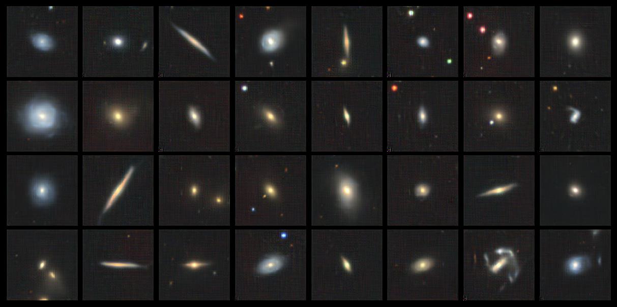
There are many datasets of galaxy images out there, but one I heartily recommend for training machine learning models is the Galaxy10 DECals Dataset, which is easily accessible as part of the astronn package. See the full details about how to access the data here.

The dataset contains colour images of size 256×256 pixels. I recommend resizing these to 128×128 pixels to get started with as the training isn’t so laborious (unless you have access to a decent, modern GPU with over 12GB VRAM, then by all means go for it).

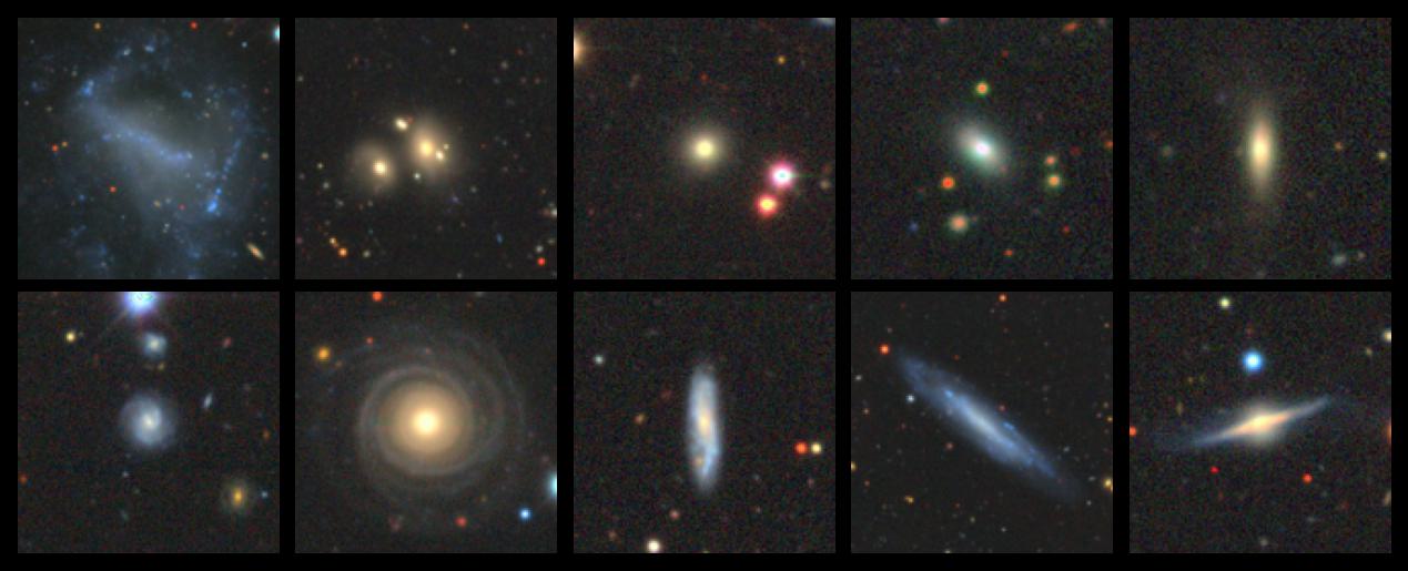
Let’s visualise some images from my GAN and see how they compare!

Not too bad for a couple of hundred epochs! But it’s clearly artificial; the most obvious giveaway being that the background considerably smoother, that the samples are somewhat more compact, and that the spirals are less well defined. It’s worth inspecting the feature maps of all the convolutional layers inside the generator to see how they “construct” the image, layer by layer, starting merely from random noise.

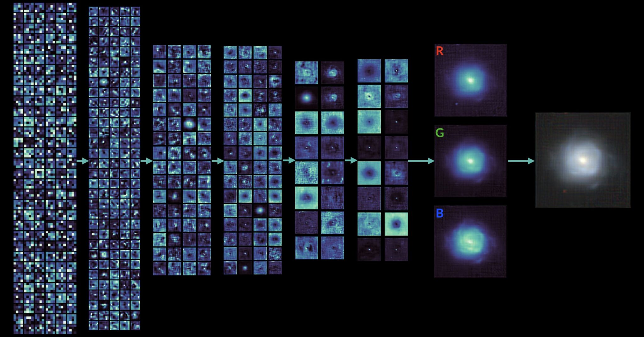
One last thing that’s worth mentioning is that the GAN we’ve discussed up to this point has been trained solely using the images without any need for labels (i.e. unsupervised learning). In other words, the generator learns to mimic the images without needing to know what the images are supposed to be. That doesn’t mean labels are useless – far from it. Suppose your dataset consists of various different categories of images, for example different types of galaxies (spiral, elliptical, etc). Since regular GANs are just trained on images regardless of type or category, they will correspondingly output images of random types: spirals, irregulars, a whole galaxy zoo. Suppose you want to force your GAN to instead output images of a specific category. To do this, we need to integrate labels into the GAN itself.

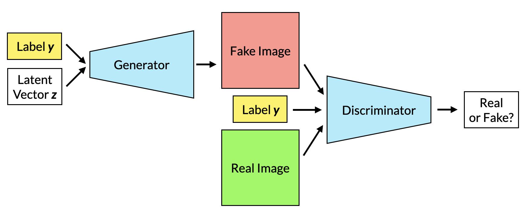
Conditional GANs

In a Conditional GAN (or CGAN, for short) (Mirza & Osindero, 2014) the images generated by the generator are now conditioned on labels. Both the generator and discriminator now accept a label as an additional input, hence their outputs are now contingent on that label. We can see this in the new loss function: \[ \min_{G}\max_{D} V(D,G) = \mathbb{E}_{x \sim p_{\text{data}}(x)} \left[\log D(\mathbf{x|y})\right]+\mathbb{E}_{z \sim p_z(z)} \left[\log(1-D(G(\mathbf{z|y})))\right] \] The generator is hence forced to generate images of different categories; so too must the discriminator correctly distinguish images of different categories. Once trained, we can use a CGAN to output different categories simply by inputting the corresponding label.

The only difference in the training loop of a CGAN as opposed to a regular GAN is that ensuring that the data is unpacked into images and labels, and ensuring that the labels are supplied to the generator and discriminator as secondary inputs). However, both the generator and discriminator must now explicitly incorporate labels.

Adding Labels

Let’s start with the generator. Because we have multiple inputs and our model is no longer linear, it’s best to use the Functional API (although you could set this up using two Sequential models). There are multiple ways to add labels; the example below uses an Embedding layer to first transform the input layer into an embedding of length 64 (this number is arbitrary). This embedding is then flattened and concatenated to the latent vector. In our case (recall the latent dimension is 128) this results in a vector of size 192.

latent_input = keras.Input(shape=(latent_dim,))
label_input = keras.Input(shape=(1,))
embedding = layers.Embedding(input_dim=10, output_dim=64, input_length=1)(label_input)
embedding = layers.Flatten()(embedding)
x = layers.Concatenate()([latent_input, embedding])
# ... regular generator code, i.e Conv2DTransform, etc
generator = keras.Model(
    inputs=[latent_input, label_input],
    outputs=outp)

In a similar fashion, the discriminator also uses an Embedding layer, the output of which is flattened, reshaped, and finally concatenated to the original input image. Thus the image now has a fourth channel representing the embedded label.

image_input = keras.Input(shape=(128,128,3))
label_input = keras.Input(shape=(1,))
embedding = layers.Embedding(input_dim=10, output_dim=128*128, input_length=1)(label_input)
embedding = layers.Flatten()(embedding)
embedding = layers.Reshape((128,128,1))(embedding)
x = layers.Concatenate()([image_input,embedding]) # shape = (128,128,4)
# rest of the discriminator code
discriminator = keras.Model(
    inputs=[latent_input, label_input],
    outputs=outp)

Synthetic Galaxies by Morphological Category

Let’s visualise the output of a CGAN trained with the 10 classes in the astronn Galaxy 10 DeCALS dataset.

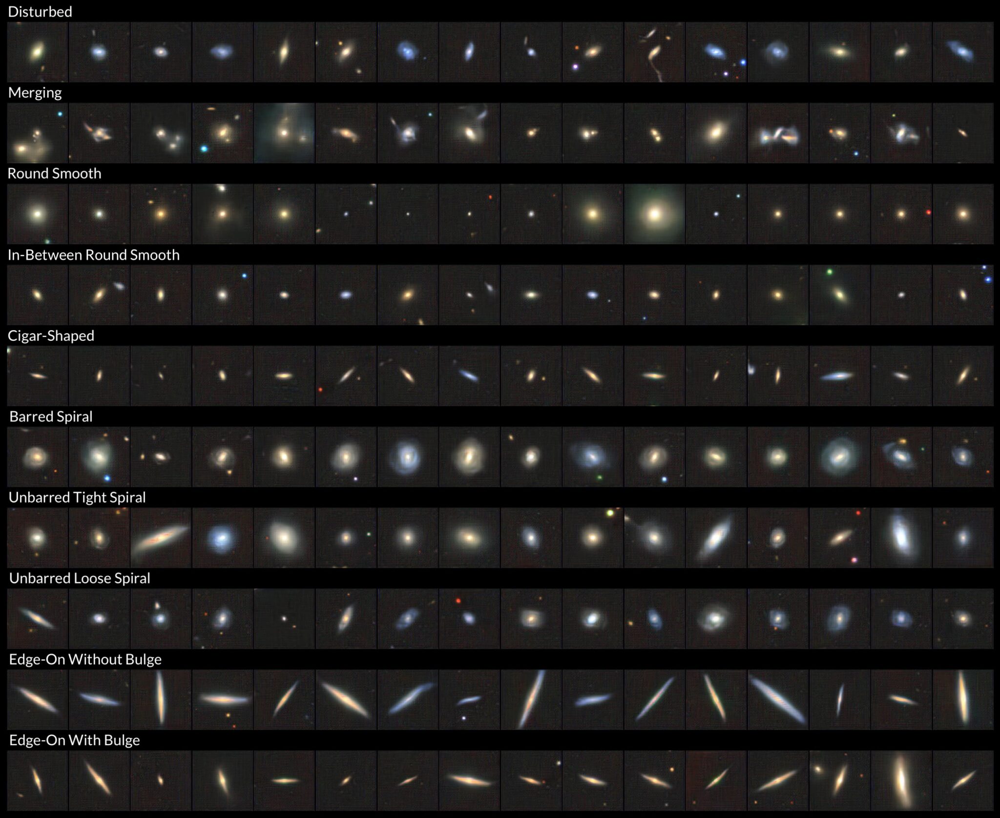
The addition of labels is a success; the CGAN is now able to output images of a desired class simply by providing the desired label.

I hope this post has piqued your interest in generative deep learning, and perhaps inspired you to delve into the wonderful world of GANs. Recent advances in large-scale, generative models, as well as natural language processing, have led to the development of models such as DALL-E Mini and Midjourney, which are capable of highly realistic image synthesis. It is humbling to think that this all stems from the fundamental ability to learn an underlying latent space best representing some arbitrary data. It seems every image on the Internet, everything supposedly “unique” in the world around us, every galaxy in the Universe, all of these are just points in a latent hyperspace. One must imagine Sisyphus happy.

References and Further Reading

• Tensorflow’s DCGAN tutorial and Keras’ extensive range of generative deep learning tutorials
• Ian Goodfellow’s seminal paper and legendary NeurIPS 2016 tutorial (talk available on YouTube)
• DCGAN original paper (Radford et. al., 2015)
• MIT’s 6.S191 Introduction to Deep Learning lecture series (especially the lecture on Deep Generative Modelling)
• https://paperswithcode.com/, perfect for keeping up with the latest advancements!

I also recommend the following books, both for GANs and for deep learning in general:

• Raff, E. (2022) Inside Deep Learning, Manning
• Chollet, F. (2021) Deep Learning in Python (2nd edition), Manning (highly recommended)
• Foster, D. (2019) Generative Deep Learning, O’Reilly
• Langr, J. & Bok, V. (2019) GANs in Action, Manning