What makes our brains tick? In particular, what allows us to make sense of what we see? To spot a familiar face in a crowd of strangers, to tell toxic shroom from psychedelic shroom, edible berry from poisonous berry, or simply to look up at the night sky and tell star from planet. Naturally, we take our ability to make sense of our world for granted, but when it comes to artificial intelligence, training a robot to perceive, interpret and respond to things within its immediate surroundings is far from effortless. The safety of self-driving cars is arguably solely reliant on image recognition algorithms. Many of the automated systems in today’s interconnected world, ranging from recommendation algorithms, Facebook advertising, Google’s real-time traffic data, business and marketing analytics, financial forecasting and more, exist because of advances in AI that stem from being able to detect patterns in large amounts of data, and being able to accurately interpret said data.
Neural networks can be considered as a family of algorithms that attempt to mimic the natural neural processes in our brains in order to train a model to interpret and make predictions about some data. Among the more celebrated neural networks of recent years are convolutional neural networks (hereafter CNNs, not to be confused with the namesake media outlet), a neural network especially suited for analysing and classifying images. They do this through a convoluted (pardon the pun) feature extraction process, which ultimately boils down to some fancy matrix algebra. Just about all neural networks boil down to fancy matrix algebra. Yet, despite the “simple” nature of CNNs, the internal feature extraction process – and the operation of neural networks in general – is often regarded as a “black box”. This is since most ready-to-go machine learning APIs just output a bunch of numbers and progress bars. One of the ways to glean some insight into what the CNN is actually doing is to have a look at the feature maps. That is what we’ll look at in this post.
So what exactly is a feature map?
This post assumes some working knowledge of CNNs, mostly terminology related. For a more in-depth overview, check out this public course material from Stanford. For the purposes of this post, let’s just briefly describe the structure and operation of a CNN. A CNN is chiefly composed of alternating convolutional and pooling layers, followed by a basic neural network of dense layers. CNNs work by first inputting an image – usually a square image, say 50x50x1 pixels or 50x50x3 for an RGB image. The convolutional layer performs a series linear convolution on the input image (through the application of initially random convolutional filters) and outputs a series of feature maps. These feature maps undergo further processing, such as further convolutions and/or downsampling in pooling layers. In general, the overall end result is our input image has now been processed into a large number of feature maps through a hierarchical-like series of convolutions and pooling. And that’s essentially the gist of what makes CNNs so powerful for image recognition.
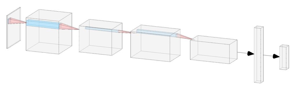
The image above, created with this excellent tool, shows a basic CNN architecture. Each “slice” of the 3D volumes corresponds to a feature map; i.e. if there are \( m \) feature maps then the dimensions of the volume are \( w \times w \times m \) where \( w \) is the size of the feature map. The last couple of layers of a CNN are so-called “Dense” layers; these are just one-dimensional arrays of nodes that are fully-connected with all the nodes in adjacent layers. The 3D volume of feature maps must first be flattened into a one-dimensional array. It is also common to include a dropout layer to ignore a set fraction of these nodes. Dropout is important to, among other things, prevent overfitting and improve regularisation.
A time-honoured example
The rest of this post will explore a very straightforward example of how to code up a CNN with TensorFlow in Python 3.X, and ultimately how to visualise the feature maps. I recommend using a Jupyter notebook to follow along if you wish. Google Colab is a great option for getting started with next to no setup.
Packages
Below is all you’ll need to follow along:
import tensorflow as tf
import numpy as np
import matplotlib.pyplot as plt
import seaborn as sn
from sklearn.metrics import confusion_matrix
As with just about every Medium or Towards Data Science article on the topic, I’ll use the MNIST dataset of handwritten digits: the “Hello world!” of CNNs. This is for good reason, as the data is built-in to Keras.
(X_train, y_train), (X_test, y_test) = tf.keras.datasets.mnist.load_data()The aim is to train a CNN to classify images of handwritten digits.
Pre-processing
Let’s first reshape the data into the correct format for loading into the CNN.
X_train = X_train[:,:,:,np.newaxis] # or alternatively X_train = np.expand_dims(X_train,-1)
X_test = X_test[:,:,:,np.newaxis]
y_train = tf.keras.utils.to_categorical(y_train)
y_test = tf.keras.utils.to_categorical(y_test)
The extra dimension is important; in general, the overall shape of the data should be (N, w, w, d) where d is the image depth (e.g. 1 for B&W, 3 for RGB). The labels are also converted into arrays of 10 elements as these are meant to correspond to probabilities. For example, a digit with the label 3 can be represented as a (zero-indexed) array of probabilities, i.e. [0, 0, 0, 1, 0, 0, 0, 0, 0, 0].
Architecture and Compilation
Let’s now code up our CNN. This will be pretty basic, just two sets of alternative convolutional and pooling layers with a single dense layer before the output.
model = tf.keras.models.Sequential([
    tf.keras.layers.Conv2D(32,kernel_size=(3,3),activation='relu',input_shape=X_train[0].shape),
    tf.keras.layers.MaxPool2D((2,2)),
    tf.keras.layers.BatchNormalization(),
    tf.keras.layers.Conv2D(64,kernel_size=(2,2),activation='relu'),
    tf.keras.layers.MaxPool2D(),
    tf.keras.layers.BatchNormalization(),
    tf.keras.layers.Flatten(),
    tf.keras.layers.Dropout(0.5),
    tf.keras.layers.Dense(256,activation='relu'),
    tf.keras.layers.Dense(len(y_train[0]),activation='softmax')
])
Here the first convolutional layer extracts 32 feature maps using a 3×3 convolutional filter (as such the size of the filter maps will be slightly smaller than the original input image). This is then passed through a MaxPool2D layer. Essentially this downsamples the image yet keeps the pixels with the highest values within the pool size (which is 2×2). Thus the dimensions of the downsamples feature maps are half that of the original. The BatchNormalization layer is not strictly necessary, but helps to enforce uniformity by standardising each set of inputs. These three layers repeat, albeit with 64 feature maps for the second convolution and with a smaller convolutional filter. Finally the feature maps are all flattened into a 1D array (with Flatten), after which 50% are ignored (this is what the Dropout(0.5) indicates). There is one Dense layer of 256 nodes, followed by the output layer which is equal to the number of output categories, in our case 10 for each of the 10 digits.
I could easily write an entire post on activation functions. For the purposes of this post, the rectified linear unit (or relu) is the standard choice for just about every layer. However, since we want our outputs to correspond to probabilities, we must use softmax. Softmax, a.k.a normalised exponential, ensures that the sum of the activations across all nodes in the layer is equal to 1.
Let’s now compile the model:
model.compile(
    optimizer=tf.keras.optimizers.Adam(lr=0.0005),
    loss='categorical_crossentropy',
    metrics=['accuracy'],
)
So we’ll be using Adam as our optimisation algorithm, categorical crossentropy to define our loss function, and our main metric will be the accuracy. Categorical crossentropy essentially looks at the difference between two probability distributions, which is important for classification tasks.
Training
Training a CNN is essentially just an exercise in mathematical optimisation, usually performed via some flavour of stochastic gradient descent algorithm. The objective is to minimise the error with the expected output (i.e. training labels) via tweaking the trainable parameters within the network itself (weights and biases). In the case of CNNs, this also includes tweaking the convolutional filters, which ultimately allow different features to be extracted from the image.
Before training we need to fix two parameters; the batch size and the maximum number of epochs. Since we don’t have infinite memory, the training data is usually randomly partitioned into various batches, with the weights and biases tweaked for each batch. Each iteration of training over all batches (i.e. over all of the data) is referred to as an epoch. It also doesn’t hurt to define some callbacks. Callbacks are functions that, by default, are triggered at the end of every epoch. One of the most useful callbacks is ModelCheckpoint, which can be used to save the best network weights to file. Another callback, EarlyStopping, is used to halt training once there is no appreciable improvement in the validation loss (by which point the network has usually overfitted to the training data).
batch_size = 200
epochs = 100
callbacks = [
    tf.keras.callbacks.ModelCheckpoint('best.hdf5',save_best_only=True,save_weights_only=True),
    tf.keras.callbacks.EarlyStopping(patience=5)
]
Now let’s train the model using model.fit. If running on Google Colab, make sure you connect to a GPU runtime.
history = model.fit(X_train, y_train, batch_size=batch_size, epochs=epochs, callbacks=callbacks, validation_data=(X_test, y_test), verbose=1)and you’ll be able to monitor the progress:
Epoch 1/100
300/300 [==============================] - 2s 7ms/step - loss: 0.2051 - accuracy: 0.9363 - val_loss: 0.0528 - val_accuracy: 0.9826
Epoch 2/100
300/300 [==============================] - 2s 7ms/step - loss: 0.0658 - accuracy: 0.9797 - val_loss: 0.0355 - val_accuracy: 0.9866
Epoch 3/100
300/300 [==============================] - 2s 6ms/step - loss: 0.0451 - accuracy: 0.9855 - val_loss: 0.0348 - val_accuracy: 0.9874
Evaluation
For the CNN above, we get
model.load_weights('best.hdf5')
model.evaluate(X_test,y_test)
which gives
313/313 [==============================] - 1s 2ms/step - loss: 0.0256 - accuracy: 0.9923

[0.025639580562710762, 0.9922999739646912]
and so our model can classify handwritten digits with an accuracy of 99.23%.
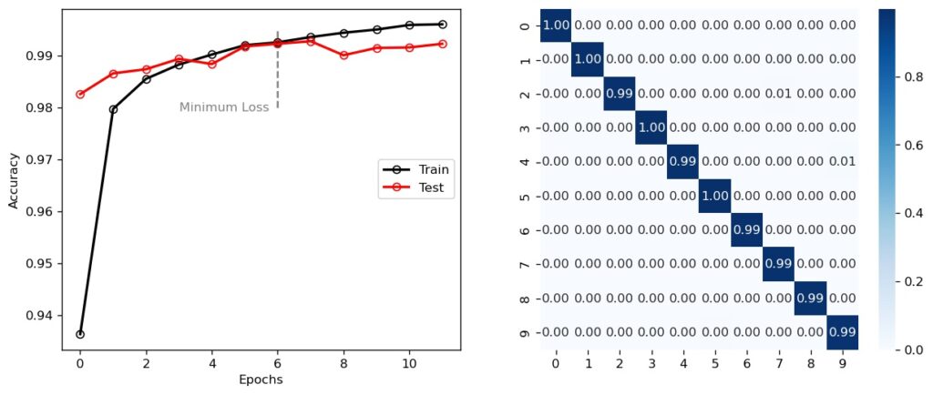
We can visualise the training history by plotting the training and testing accuracies over time. We can also plot the confusion matrix (or error matrix), where each cell \( (i,j \) gives the fraction of samples with true label \( i \) and predicted label \( j \). For a perfect CNN, a confusion matrix should equal the identity matrix and, as we can see below, that is pretty much the case with this CNN. The only significant blips are the 1% of 2s misclassified as 7s, and the 1% of 4s misclassified as 9s.
Aside: A note on data partitioning
A complete dataset is usually partitioned into at least two separate sets for training a neural network: a training set (with which to train) and a testing set (with which to validate and evaluate). That’s essentially what we’ve done, yet a hawk-eyed reader would no doubt see the parameter “validation_data” in model.fit. It’s important to note that the parameter just refers to some data that, in turn, is used to calculate the val_loss and val_accuracy values. The reason I bring this up is that you may have read, or indeed use, three separate partitions of the data; a training set, validation set and testing set. Our current testing set is essentially also our validation set; we are using it to evaluate the performance of the CNN…
BUT, if we were to go back and change the architecture of the CNN, and we wish to properly compare the new CNN with the old CNN, we need to have a third, independent set of data that is unseen by both CNNs. Any changes we make to our current CNN are essentially biased to the data we’re currently using to evaluate it. To remove this bias entirely, we must use a third, independent set.
In normal usage this technicality is too small to worry about, but if you want to rigorously compare different CNNs then you need to ensure that you have an independent set of data to test on. One quick way to do this with the data we’ve got is to just halve the existing X_test array into an X_val and new X_test array. Then you’d evaluate the CNNs with X_val and, once you’ve modified the architecture to your liking, perform a final test with X_test .
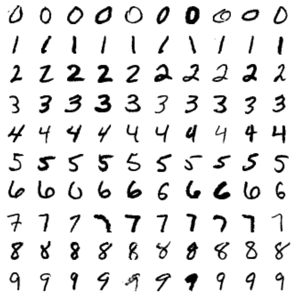
Let’s see how well the CNN performs by plotting 100 example digits, 10 per row, that the network has classified as \( 0, 1, 2, \ldots \):
Feature Maps
Let’s now get to the heart of what this post is about; visualising the feature maps. There is no in-built way to do this in Keras, but it’s fairly straightforward to define a new model that we can use to extract the activations of each feature map (and thus plot them).
activation_layers = [i for i in model.layers if ('conv' in i.name or 'pool' in i.name)]
activation_model = tf.keras.Model(
    inputs = model.inputs,
    outputs = [i.output for i in activation_layers]
)
feature_maps = activation_model.predict(image)
Here the image should be some array with the shape (1, w, w, 1), like X_test[0,:,:,0], i.e. the first image in the X_test array. From here you can obtain the individual feature maps for a given layer as follows. Here is an example for the first convolutional layer (in this case feature_maps[0])
nmaps = feature_maps[0].shape[-1]
fig = plt.figure(figsize=(8,4),dpi=120)
for i in range(nmaps):
    fig.add_subplot(4, 8, i+1)
    plt.imshow(feature_maps[0][0,:,:,i],cmap='binary')
    plt.axis('off')
plt.show()
Let’s see an example with a random number 8.

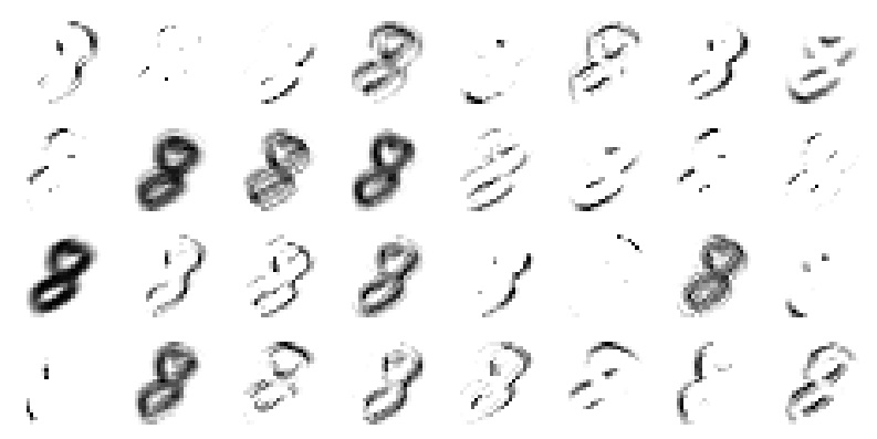
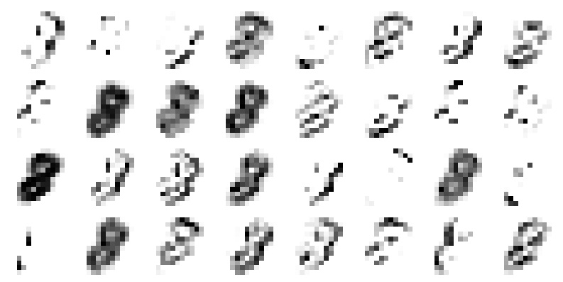
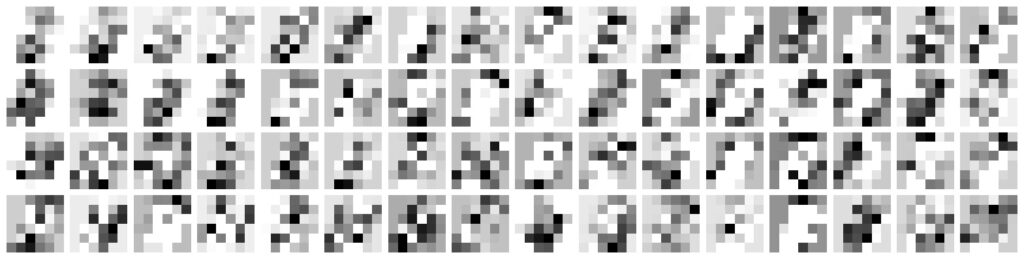
By the time the image has progressed through to the final pooling layer before flattening, the image is barely recognisable. Nevertheless, it is these “features” that the CNN has learned, through training, to recognise as an image of a handwritten 8. Indeed, the first convolutional layer demonstrates how the input image is transformed via linear convolutions into 32 feature maps, with various combinations of edge detection, blurring and smoothing. This should come as no surprise as linear convolutions are the same fundamental process that GIMP and Photoshop use for applying image effects. Remember, it all boils down to fancy matrix algebra.
We could get into all sorts of metaphysical and/or philosophical arguments about whether these feature maps are the AI equivalent of what our visual cortex does, but there’s no denying how truly effective CNNs are at image classification tasks. So effective that an entire, burgeoning subfield of AI, deep learning, is devoted to the research and development of far more intricate networks, which have applications in myriad disciplines including machine translation, speech recognition and dictation, bioinformatics and pharmaceutical research, autonomous vehicles, medical imaging, data analytics and even in planetary science and astronomy.
You’ve probably run into deep learning without even thinking about it. Your Google searches, all the ads and/or warnings for fake news you see on social media, filters you put on your videos to make yourself look better, virtual chatbots when online shopping, Netflix recommendations on what to watch next, Spotify’s Discover Weekly, interactions with Siri and, for those who can actually get a damn RTX 3000 series card, video game graphics. Neural networks, and AI in general, will play a significant role in shaping our technological future. Hopefully this post has given you an idea of how CNNs process and “see” image data.
Resources
The official TensorFlow website, along with Google’s own crash course, have some excellent tutorials.
I also highly recommend 3Blue1Brown’s videos on the topic of neural networks, which give an outstanding conceptual overview of how neural networks work at the fundamental level.
Another great resource is the free online book by Michael Nielsen titled Neural Networks and Deep Learning, in particular for its mathematical treatment of back-propagation.
Turing Award laureate Yann LeCun’s seminal 1998 paper on document recognition and influential 2015 Nature paper on Deep Learning are excellent resources to delve deeper into CNNs and other types of neural networks.