Nothing heralds Christmas and the end of the year more than the World Darts Championship. It’s also that time of the year when I commit to actually creating a script to generate all possible legal checkouts from a given score (e.g. checkout(170) should return ['T20', 'T20', 'BULL']), only to not actually have time to do so, because it’s Christmas and New Years and Steam Sale time. In this post, I’ll discuss calculating the number of ways to checkout via two methods: depth-first search and dynamic programming.

In the first method, we construct a path to checkout one dart at a time (starting with the first dart thrown and last dart thrown) using a depth-first search. This can be thought of as a “top-down” approach. The second method is instead a “bottom-up” approach: we start from the last dart back up to the first dart by gradually populating a matrix. This is one of the principles of dynamic programming. We’ll discuss the drawbacks of depth-first search (and exponential algorithms in general) and methods to improve its performance. Lastly, we’ll demonstrate how dynamic programming cuts through the issues of exponential search, thus being overwhelmingly more efficient (albeit not without caveats).

Darts and Checkouts

In darts, players take turns throwing darts onto a dartboard such that each dart scores points according to the region in which it lands. A dartboard is subdivided into 20 segments, numbered 1 to 20, with an outer double ring, inner triple ring, and a central bullseye surrounded by another ring. Darts landing in the double ring double the score for that segment (ditto for triple ring), while the bullseye is worth 50 points, with the ring surrounding the bull worth 25 points. Each player throws three darts per turn, and so the highest possible score one can achieve in any turn is 180.

In this post I will refer to a dart as its string representation, e.g. T20 is a dart landing in the triple ring in the segment numbered 20 (worth 60 points), D12 is a dart landing in the double ring in the segment numbered 12 (worth 24 points), 16 just refers to a dart landing in the segment numbered 16 (worth 16 points), and so on. According to this definition, there are 62 unique darts, worth 43 unique points. This is since some scores, e.g. 18, can be scored with more than one dart (T6, D9 or 18).

In a typical game, players start on 501 points and must win by performing a checkout, i.e. the final dart must land on a double (including the bullseye). One of the great moments in darts is seeing a player perform difficult checkouts, or missing their first dart and having to do rapid mental math to come up with another checkout. This is where it’s fun to watch the live coverage display the ever-changing checkout combinations (at least for me it is). Let’s now consider how you might go about coding that.

One trivial way to implement this is to simply randomly choose X darts, add up their values, and see if the total equals the desired checkout score with at least one of the darts being a double (or bullseye). This avoids any need to hard-code anything, but as it is inherently probabilistic it will require a very, very large number of iterations in order to sample all possible dart combinations. A better method is to use a recursive depth-first search.

The Top-Down Approach

Depth-first search is one of the major search algorithms for exploring a graph. In the case of dart combinations, we are actually constructing a tree, with the root node being the dart we threw first, with that node’s children being the possible darts we could throw next, and so on and so on. The depth of the tree is simply the number of darts thrown, while the breadth is the number of possible darts to throw. As such, the complexity is \( \mathcal{O}(b^d) \).

In Python-flavoured pseudocode, we could do something like this

checkouts = set()
def calculate_checkout(score, maxdarts, darts)
  if maxdarts == 0:
    return
  for dart in (darts to throw next):
    if value of darts+dart == score:
      checkouts.add(tuple(darts+dart))
      return
    else
      calculate_checkout(
        score = score - value of dart
        maxdarts = maxdarts - 1
        darts = darts + dart
      )

Ways to Checkout

Now we’ve got some code, let’s explore some darting statistics. In particular, let’s plot the number of ways you can checkout in a single turn (i.e. with at most 3 darts) for a given score.

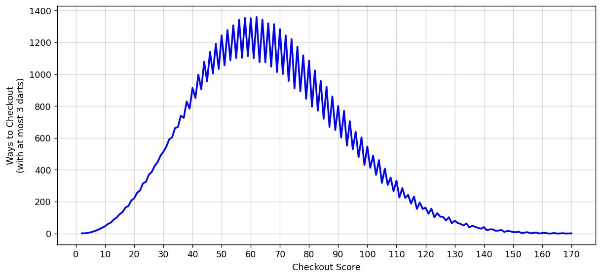
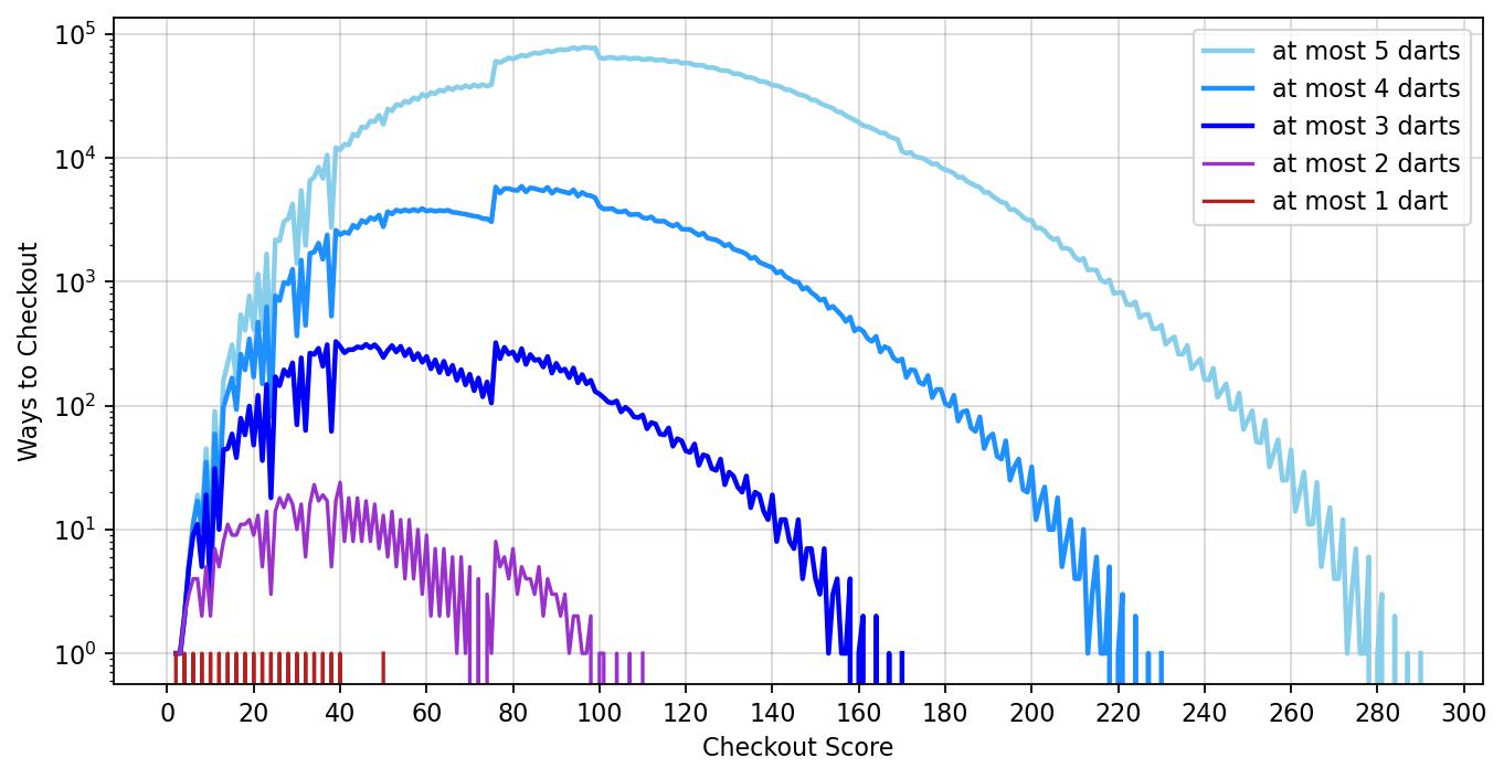
We get a somewhat skewed normal distribution, with quite a bit of oscillatory behaviour (alternating between even and odd scores). We’ve plotted the number of ways to checkout with at most 3 darts. How about at most 2 darts? Or a single dart (which, let’s be honest, is trivial)? It’s worth plotting all these three in order to visualise a most intriguing pattern (note the logarithmic scale on the y-axis).

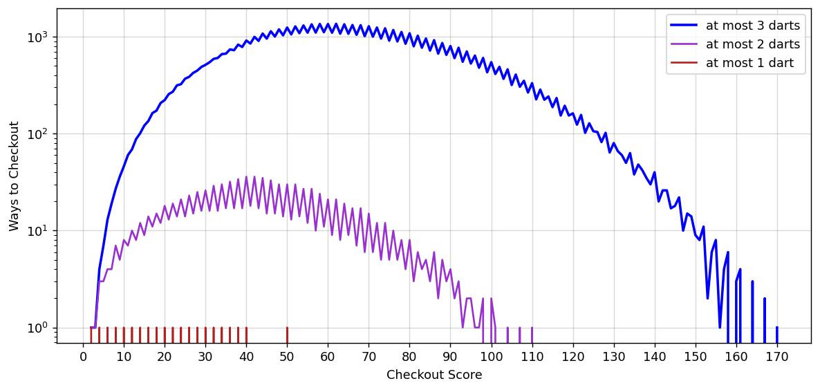
From here it’s quite easy to see the maximum scores on which to checkout with at most N darts. For one dart that’s simply the bullseye (50). In the case of 2 darts, the highest checkout is 110 (T20+BULL), and in the case of 3 darts the highest checkout is 170 (T20+T20+BULL), from which it’s clear that for \( N \) darts the highest checkout is \( (N-1)\times 60 + 50 \). A more interesting quantity is the score with the most ways to checkout on, which for the 2-dart case is both 40 and 42 (tied at 36 ways) and 62 for the 3-dart case (1360 ways).

Doesn’t that depend on how “way” is defined?

Wait, I hear you asking. How have I defined “ways”? Consider a sequence like T20+T19+BULL. If, instead, the player decided to throw the T19 first, and so ends up throwing T19+T20+BULL, should that be treated as a separate “way”? As of now (and implied by the pseudocode) the code considers these to be different ways as they are in a different order. If instead we define a “way” as a unique sequence where order doesn’t matter, then T20+T19+BULL and T19+T20+BULL are equivalent and hence correspond to only one unique way.

You may be tempted to think this is just a mere technicality, but this change in definition actually has a striking impact on the distribution of the number of ways to win. Consider, now, the 3-way case:

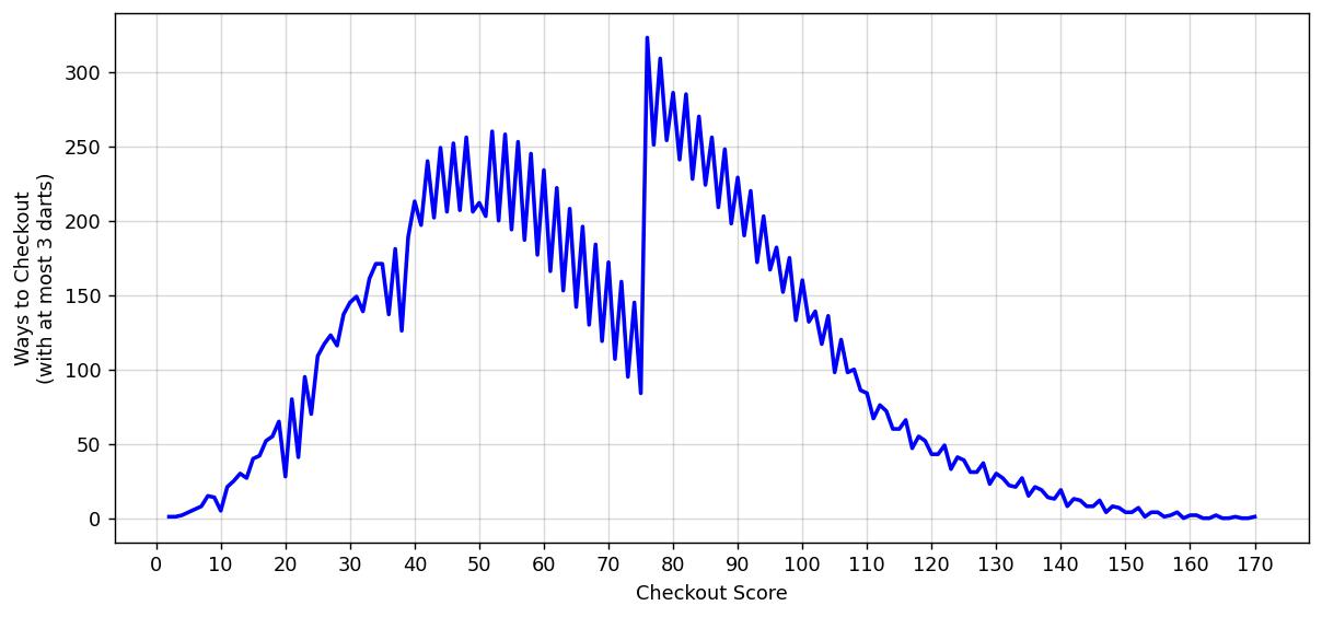
The distribution now has a large kink near the middle. Furthermore, the score with the most ways to win with at most 3 darts is now 76 (323 ways). This doesn’t just affect the 3-dart case, let’s now re-plot Figure 2 with the new definition of a “way”:

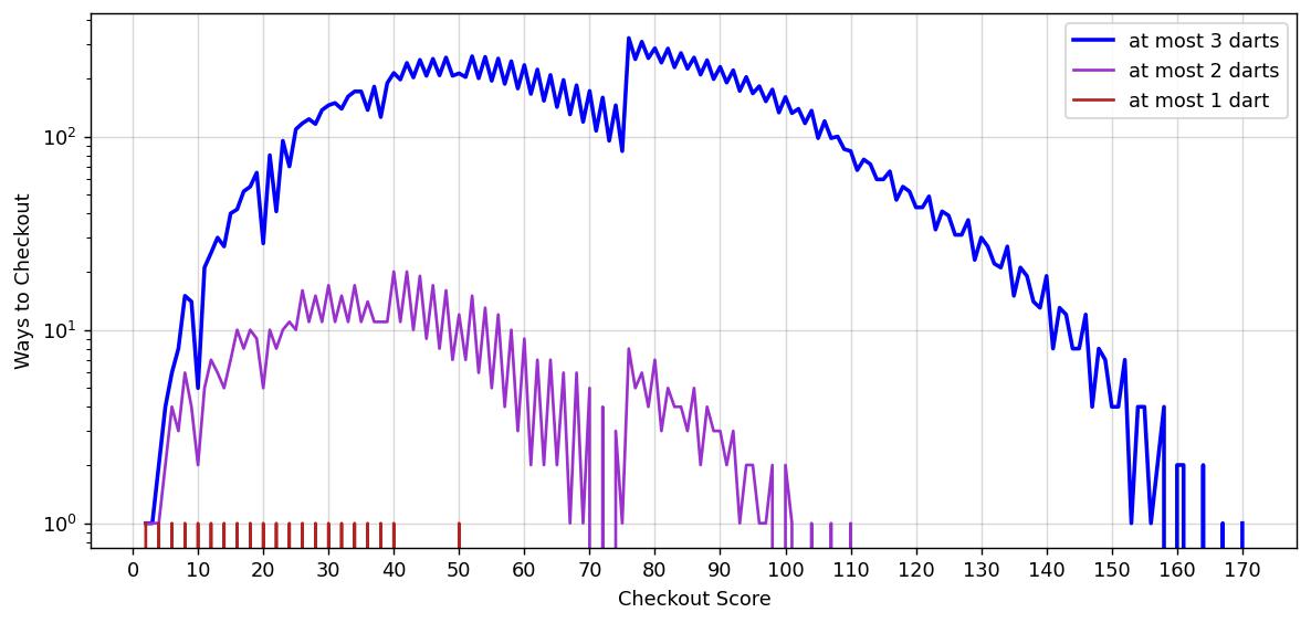
For the rest of this post, we will adopt the definition that a “way” to checkout must be unique, i.e. the order does not matter, only the darts themselves.

The Bane of Exponentials

As aforementioned, the highest value one can checkout on with at most 3 darts is 170, achieved by throwing T20+T20+BULL. This is the only solution for 3 darts. What if we could checkout from 170 with at most 4 darts? Turns out there are 327 unique ways to checkout from 170 with at most 4 darts. How about at most 5 darts? 19,701 unique ways. We could go on and on to find the number of ways for an arbitrary number of darts. However, there is a big problem. Consider the following table:

Score	# of Darts	# of Checkouts	Running Time
170	3	1	0.6 sec
170	4	327	2.3 sec
170	5	19701	2 min, 22 sec

The running time for the 5 dart case has exploded! That’s because the search space is exponential, in particular for the 5 dart case the code has to evaluate \( 62^5 \approx 916,132,832 \) possible combinations. If we were to evaluate the 6 dart case, we’d have 56,800,235,584 possible combinations to evaluate, which would take at the very least 2-3 hours (probably a lot more) to evaluate. This is, of course, the reason why exponential algorithms are a nightmare, and also why depth-first search quickly becomes intractable for deeper searches.

Pruning the Search Tree

The complexity of depth-first search is \( \mathcal{O}(b^d) \). So, for a fixed depth \( d \), one way to improve running time is to try and reduce the breadth of the search (i.e. to trim or prune the search tree). We are looking at all 62 darts each time. What if we didn’t have to? Indeed, we shouldn’t have to. One relatively simple restriction is to just throw trebles when the remaining score is high. After all, on the path to completing 170, why would you throw a 1? This is a reasonable restriction to implement when the remaining score is above 100 as all scores above this must require a treble. Furthermore, why throw trebles when the score is low? We can reasonably restrict the choice of darts to singles and doubles for scores less than or equal to 75 (of which 25+BULL is the highest checkout for 2 non-treble darts). More concretely, it’s worth only choosing darts whose value is less than the current score, which seems like an obvious conclusion, but is especially useful for very low scores where we can ignore heaps of doubles. We could further refine this with more aggressive pruning, such as by restricting trebles to just commonly-thrown ones 'T20', 'T19', 'T18', etc, and completely discarding low-value darts like 1, D1, 2, D2 when the score is still high. Implementing these changes lead to the following results:

Score	# of Darts	# of Checkouts	Running Time	Speedup
170	3	1	0.2 sec	3x
170	4	216	0.6 sec	4x
170	5	9195	0.8 sec	177x
170	6	158524	27 sec	300x (est.)

That’s right! Having pruned the search tree, it’s now possible to compute the result for the 6-dart case in well under a minute instead of potentially several hours! It’s worth noting that because we’ve pruned the search space, the search is no longer exhaustive and so the number of checkouts able to be found is less than the actual number of possible checkouts. As with so many things in life, a faster solution often sacrifices completeness.

I should note that the method as-is is still quite wasteful as there are many duplicated calculations. A much more computationally efficient implementation would involve storing the results of known checkout combinations in a table (i.e. memoization). Suppose after throwing some darts the score is now 78. Instead of recursively branching from 78, we could instead see if we’ve already found an optimal path from 78 (say T18 and D12) and just fetch this result from the existing table rather than recomputing everything. While this is certainly best in practice, it does mean you’ll be stuck on the same combination pathways and hence miss a lot of valid checkouts. For example, if 'T18', 'D12' is listed as the only entry for 78, all future pathways will default to this. Hence other checkouts like 'T14', 'D18' and 'T20', 'D9' , while perfectly valid, won’t be considered. No doubt the actual darts checkout program used for televised darts would incorporate a weighted probability for these checkout combinations based on the difficulty of the checkout, as well as the chance of being able to resort to a fallback “Plan B” checkout should the first dart miss. In this way, the table only needs to store the checkouts “most likely to be played” rather than all possible checkouts.

Ways to Checkout II

With these optimisations in place, we can look at ways to checkout with more than 3 darts. Let’s plot darts up to 5. Note, again, the logarithmic plot.

It’s interesting to see how the shape of the distribution is stretched as the number of darts increases. In particular, for the 2, 3 and 4-dart case we see the gradient of the curve decreases at the major kink at checkout score 76, while for the 5-dart case the curve continues to increase. Also note that, even despite the optimisations, we can’t escape the fact that the code is inherently an exponential algorithm. The ways to checkout grows by at least an order of magnitude as the number of darts increases.

There are only 18 unique nine-darters

9-dart finishes are incredibly rare, requiring a 180 first up and perfect play with no mistakes from then on. If you Google “how many ways to score a 9 darter”, you’ll get various values ranging from 1,000 to 3,944. As we will see, there are indeed 3,944 ways to score a 9-darter, but I contend that of these, only 18 are unique:

('T20', 'T20', 'T20', 'T20', 'T20', 'T20', 'T20', 'T19', 'D12')
('T20', 'T20', 'T20', 'T20', 'T20', 'T20', 'T20', 'T17', 'D15')
('T20', 'T20', 'T20', 'T20', 'T20', 'T20', 'T20', 'T15', 'D18')
('T20', 'T20', 'T20', 'T20', 'T20', 'T20', 'T19', 'T18', 'D15')
('T20', 'T20', 'T20', 'T20', 'T20', 'T20', 'T19', 'T16', 'D18')
('T20', 'T20', 'T20', 'T20', 'T20', 'T20', 'T19', 'D17', 'BULL')
('T20', 'T20', 'T20', 'T20', 'T20', 'T20', 'T18', 'T17', 'D18')
('T20', 'T20', 'T20', 'T20', 'T20', 'T20', 'T17', 'D20', 'BULL')
('T20', 'T20', 'T20', 'T20', 'T20', 'T19', 'T19', 'T19', 'D15')
('T20', 'T20', 'T20', 'T20', 'T20', 'T19', 'T19', 'T17', 'D18')
('T20', 'T20', 'T20', 'T20', 'T20', 'T19', 'T18', 'T18', 'D18')
('T20', 'T20', 'T20', 'T20', 'T20', 'T19', 'T18', 'D20', 'BULL')
('T20', 'T20', 'T20', 'T20', 'T20', 'T17', 'BULL', 'BULL', 'BULL')
('T20', 'T20', 'T20', 'T20', 'T19', 'T19', 'T19', 'T18', 'D18')
('T20', 'T20', 'T20', 'T20', 'T19', 'T19', 'T19', 'D20', 'BULL')
('T20', 'T20', 'T20', 'T20', 'T19', 'T18', 'BULL', 'BULL', 'BULL')
('T20', 'T20', 'T20', 'T19', 'T19', 'T19', 'T19', 'T19', 'D18')
('T20', 'T20', 'T20', 'T19', 'T19', 'T19', 'BULL', 'BULL', 'BULL')

All other paths to checkout are just permutations of the above 18 (whether you consider separate permutations to count as a separate way is ultimately subjective!) Indeed, there is nothing stopping you from throwing these in any order so long as the final dart is a double. Good luck landing three bullseyes, though.

The Bottom-Up Approach

As we saw, a depth-first search is time consuming, and even with a pruned search tree, increasing the depth of the search leads to considerably higher running times. There is another approach to calculating the number of ways to checkout, and it’s a fairly simple recursive matrix calculation.

Suppose we have a matrix of size \( d \times s \) where \( d \) is the maximum number of darts to be thrown and \( s \) is the highest score to calculate from. Without loss of generality, let this matrix be of size \( 3 \times 170 \). Each element \( [i, j] \) of the matrix thus represents the number of ways to checkout from score \( j \) using \( i \) darts. Clearly, we want the entry \( [3, 170] \) to equal \( 1 \). How can we go about populating this matrix?

First, let’s populate the entries in the first row, i.e. \( i = 1\). By definitions, the only scores that can be checked out from with just one dart are the doubles including bullseye, so we can quickly go and set \( [1,2] = 1, [1,4] = 1, [1,6] = 1, \ldots, [1,50] = 1 \). All other numbers are just set to \(0\). The next step is to populate the second row, i.e. \( i = 2 \). The following formula should do the trick: \[ M_{i,j} = \sum_{d \in D : d < j} M_{i-1,j-d} \] where \( D \) is the set of darts whose value is less than \( j \). That is, the value of the matrix at \( [i,j] \) is simply equal to the sum of the values in the previous row \( i-1 \) with scores obtained after throwing a legal dart \( d \).

Populating a matrix through splitting some problem into multiple sub-problems, and then recursively combining the solutions to these sub-problems to construct the solution to the original problem, is one of the key concepts behind dynamic programming. Not all problems can be solved with dynamic programming as there must inherently be some sort of recursive substructure. Perhaps the best example of a problem with recursive substructure is the Towers of Hanoi puzzle, but when it comes to dynamic programming you may also have heard of the 0-1 Knapsack problem. It’s fairly intuitive, in the case of darts, to find a recursive substructure. For instance, the number of ways to checkout from 170 with 3 darts must be related to the number of ways to checkout from 110 with 2 darts (if, say, we threw a T20). Indeed, it’s related to the number of ways to checkout with 2 darts from all possible scores that can be reached with 1 dart starting from 170. This is why we must sum the \( M_{i-1,j-d} \) term for all darts \( d \) (the condition \( d < j \) is to prevent negative scores).

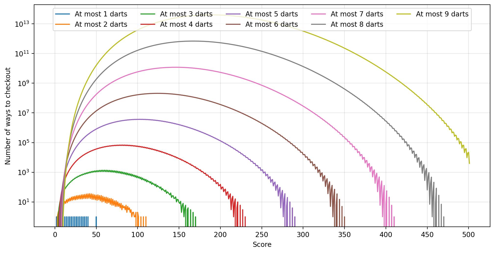
This method is insanely more efficient than a depth-first search, and allows us to rapidly visualise the number of checkouts up to 9 darts in mere seconds (0.7s according to VS code). The only limit to the depth is ultimately integer overflows since, as can be seen in Figure 7, the number of ways grows exponentially. However, unlike a DFS, it does not directly yield the actual dart combinations. These are difficult to calculate based purely on the matrix of values without resorting to a pseudo-recursive depth first search (in which case you’re probably better off doing a depth-first search anyway).

Lastly, as a quick sanity check, we find that matrix[3,170] = 1 and matrix[9,501] = 3944, just as expected.