If you’re like me and you feel the need to come up with fantasy maps on the fly every now and then, you might take to a piece of paper and scribble some landforms. Alternatively, you could load up GIMP (or Photoshop if you’ve got plenty of disposable income), make some random clouds, apply a threshold, and drag until you have some suitably aesthetic fractal terrain. Let’s see if we can do the same thing using just your favourite programming language.
The Diamond and the Square
One of the simplest ways to generate a so-called cloud or plasma fractal (and hence fractal terrain) is to use the diamond-square algorithm. Essentially, this algorithm is used to create a heightmap by populating a 2D matrix with random values, starting with the corners of the matrix which are set to some initial seed. Let us illustrate the basic steps using the trusty Wikipedia image.

The first step is to fix the corners of the matrix to some initial, random seed. Next, we apply the diamond step (2nd panel of Fig 1). In this step, we set the value of the midpoint of the square to the average of its four corners plus a random value. In particular \[ x_{(i_c, j_c)} = ( x_{i_0,j_0} + x_{i_0, j_1} + x_{i_1, j_0} + x_{i_1, j_1} ) / 4 + m \times r \] where \( (i_c, j_c) \) are the coordinates of the midpoint of the square defined by top-left corner \( (i_0, j_0) \), height \( j_1 – j_0 \) and width \( i_1 – i_0 \) where \( i_0 < i_1, j_0 < j_1\). Here \( r \) is a random value and \( m \) is the roughness value. The idea is that with a larger value of \( m \) the terrain is much more jumpy and random, while a smaller value yields smoother terrain.
Next comes the square step (3rd panel of Fig 1), where we now look at the 4 midpoints of the sides of the square and set these to the average value of its adjacent points plus a random value. The four midpoints are \( (i_c, j_0), (i_c, j_1), (i_0, j_c) \) and \( (i_1, j_c) \). For each of these points \( (i,j) \), we simply set its value to the average of the points \( (i-s, j), (i+s,j), (i,j-s) \) and \( (i,j+s) \) where \( s \) is the half-length of the edge (i.e. the arrows in the 3rd panel of Fig 1), plus a random value. Now, the hawk-eyed reader will no doubt realise that some of these points do not actually exist. This occurs during the first application of the square step, and in subsequent square steps for points at the edge. There are a few ways to resolve this:
- Just use 3 points instead of 4
- Count the innermost point twice
- Wrap the outermost point to the other side of the square (this actually causes more problems than it solves, as most of the time the other point has not actually been initialised)
- Give up
My personal recommendation is to count the innermost point twice, but you’ll definitely find other guides advocating for using 3 points and/or wrapping (or calling it a day). Once the square step is complete, we repeat the diamond step, but this time for each of the new, smaller squares (see 4th panel in Fig 1). The diamond and square steps alternate until the entire matrix is complete.
You cannot apply the diamond-square algorithm to an arbitrarily sized matrix. In Fig 1 the diamond and square steps are applied twice. The final step must be a square step, and a combination of the diamond and square steps always results in a new square that is at least half the size of the old square. In other words, what we have is an exponential algorithm, and the matrix must be a square matrix with side lengths equal to \( 2^n + 1 \) where \( n \) is the number of iterations of diamond steps (or square steps). A 7×7 matrix cannot work as the diamond step leaves four new 4×4 squares.
So what random values should you use?
It’s really up to you, as all this does is modify the overall look of the fractal terrain. However there is one requirement that the roughness \( m \) should decrease every time we iterate to the next sub-square (i.e after one “loop” of the diamond-square steps). This can be a linear or exponential decline. As for the random values, some advocate for using strictly positive values between 0 and 1 while others suggest going between -1 and 1. Go with whatever looks best, or rather what most suits what you are looking for.
Examples
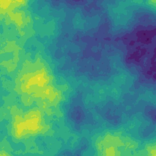
Here is an example of a cloud fractal generated with the diamond square in Python and plotted with plt.imshow with the default “viridis” and “terrain” colormaps (for contrast):
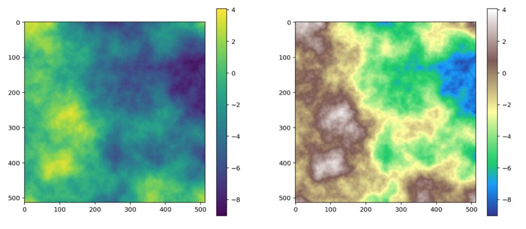
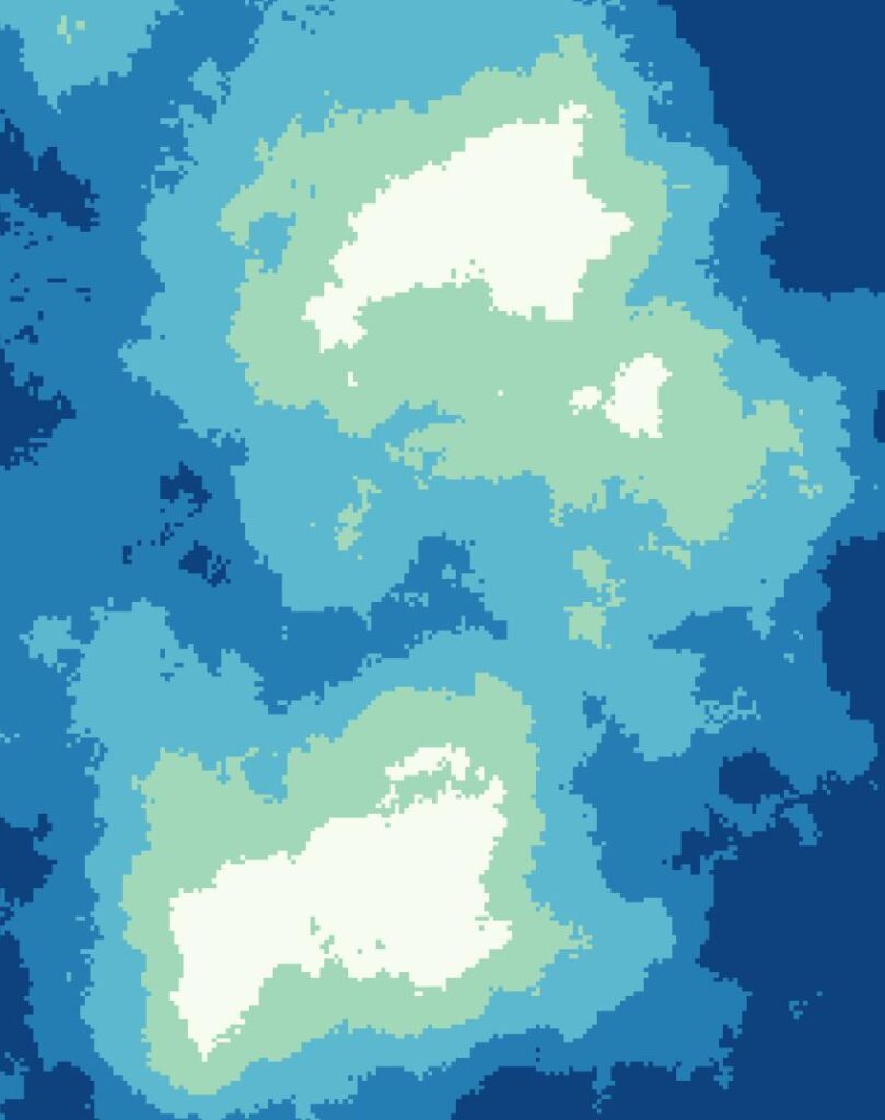
Of course, a heightmap is just a heightmap, these values can be anything you want them to be. The blue need not be an ocean, the white need not be a mountain peak. One way to better visualise the look of the terrain is to round every value in the matrix to say the nearest whole integer (for finer detail you may consider rounding to the nearest multiple of 2, 5, tens unit, etc).
We can then go and select whatever slice of the terrain looks nice (here I just used np.where to select and add up different heights in the terrain).
Nicer Example
I found the Gondwana-Laurasia continental map in Fig 4 at little too uninspiring and too rigid, so I chose the following example to better illustrate the fractal nature of the diamond-square algorithm.
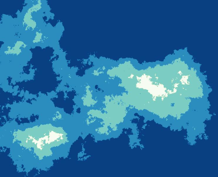
Of course there’s nothing to stop you from prettying this up / tracing the contours using Inkscape (or Illustrator if you’ve got plenty of disposable income), and lo’ and behold you’ve got a fantasy map! Now all that’s left is to write the accompanying fantasy novella.