A convolutional neural network (CNN) is a type of neural network especially well-suited to processing images. They have been the bedrock of countless deep learning applications throughout the last decade, including my current PhD research on the morphological evolution of galaxies. When talking about the technical aspects of my research, one problem I’ve encountered is how to effectively convey exactly what a CNN is doing. While it’s clear what’s happening mathematically, equations hardly make for exciting Keynote presentations, nor are the concepts themselves immediately intuitive. This is why being able to visualise what the CNN is doing is helpful.
In my previous post on CNN visualisation, I focused on plotting the feature maps of a fairly mundane CNN trained on the MNIST handwritten digits dataset. In this post I’ll revisit feature maps, but also venture further and explore the convolutional filters (both filter weights and filter patterns via gradient ascent). Rather than just using MNIST again (and becoming yet-another-MNIST-blog-post), it’s high time I showcased one of my own CNNs, trained to classify galaxies. This post assumes a familiarity with neural networks, however I will introduce the core concepts and terminology necessary for this post in the section below. Code examples are in Python and use tf.keras.
Convolutional layers
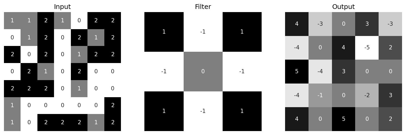
At the heart of all CNNs are the convolutional layers, which are used for feature extraction. Each layer consists of several, learnable filters (a.k.a kernels). Input images are convolved with these filters in order to produce unique outputs. Consider the following example:
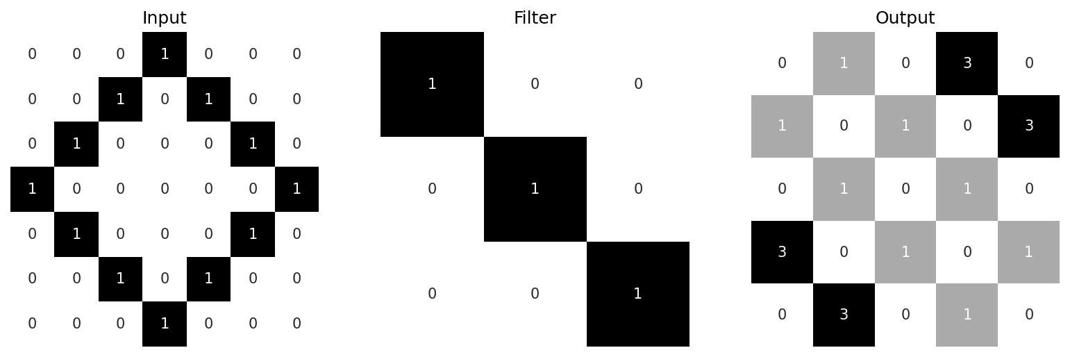
Here, our input is a 7×7 pixel image, and our filter/kernel is a 3×3 identity matrix. The image is convolved with this filter, producing an output feature map (a.k.a activation map) that highlights the top right and bottom left edges of the diamond. The convolution operation proceeds as follows. In each step, the filter “scans” a region of the image and multiplies (element-wise) the values of the pixels with the values of the filter weights, then outputs their total sum plus a bias. Note this operation is different to regular matrix multiplication. In the example above, the layer processes 3×3 windows of the input starting from the top left: the first calculation is \[ \begin{bmatrix} 0 & 0 & 0 \\ 0 & 0 & 1 \\ 0 & 1 & 0 \end{bmatrix} \ast \begin{bmatrix} 1 & 0 & 0 \\ 0 & 1 & 0 \\ 0 & 0 & 1 \end{bmatrix} = 0\] which gives us the top-left value in the output (in this example there is no bias). Output values are also known as activations, and the overall output is often collectively referred to as the activation. We then shift over by one column and look at the next 3×3 window \[\begin{bmatrix} 0 & 0 & 1 \\ 0 & 1 & 0 \\ 1 & 0 & 0 \end{bmatrix} \ast \begin{bmatrix} 1 & 0 & 0 \\ 0 & 1 & 0 \\ 0 & 0 & 1 \end{bmatrix} = 1 \] Once we reach the final column, the window returns back to the first column and is shifted down by one row. The number of rows/columns to shift over is known as the stride. In this example it’s just 1 (for both columns and rows) but it’s not uncommon to use larger strides. This process continues until the entire image is processed and the output matrix is fully populated. See the additional examples below:
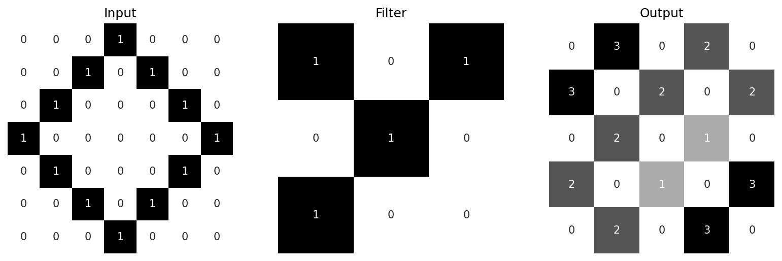
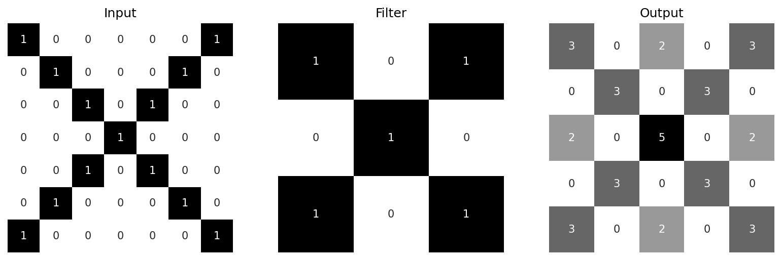
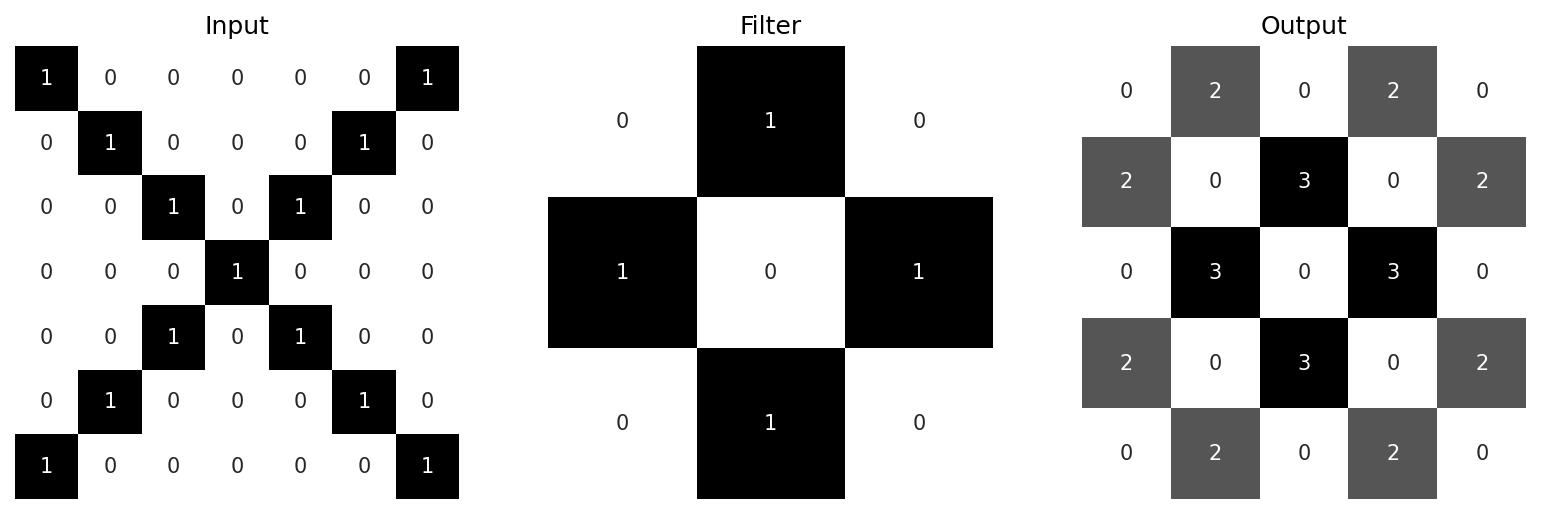
The key idea of CNNs is that these filters are learnable. Their weights start out completely random, but are tweaked over time as the model is trained. This is how CNNs are able to extract meaningful features from data. Note in these examples the feature maps are all smaller than their inputs. It’s often desirable to add padding to the input image so that the outputs remain the same size. The convolution operation can also be tweaked with different strides and even utilise dilation (where a kernel is expanded by inserting zeroes between its filter weights), but that’s beyond the scope of this particular post.
To summarise the key definitions, convolutional filters apply sets of learnable filter weights in order to extract meaningful features from data. The outputs of a convolutional layer are called the feature maps. It’s also possible to visualise the patterns of convolutional filters by crafting an input image that most strongly activates it – more on this towards the end.
Feature maps
As discussed above, feature maps refer to the outputs of convolutional layers. They are also referred to as “activation maps”, “intermediate activations” or “intermediate outputs” in a more general sense to refer to outputs of layers within the model (as opposed to the model’s final output). Below is a plot showing a selection of feature maps in all five convolutional layers (plus the final pooling layer) of one of my galaxy CNNs. The leftmost column shows the input images, which consist of five galaxies: one for each morphological category. This is followed by the convolutional and pooling layers. The final column shows the output probabilities for each class. The elliptical, spiral and edge-on images are confidently classified. The lenticular and irregular examples are also correctly predicted, however in both cases the model has also assigned a smaller probability to the “spiral” class.
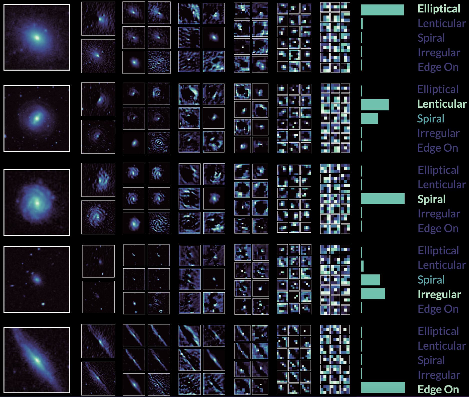
One of the key ideas of deep learning is the notion of abstraction. As illustrated above, the more convolutional layers we add, the more abstract the feature maps become, until by the final pooling layer the feature maps might as well be random noise. This hierarchical approach to abstraction allows the model to obtain highly compressed yet meaningful representations of data.
You can extract the intermediate output of any arbitrary layer in a keras.Model object as follows:
model = myModel() # your CNN model here
# ...
feature_model = keras.Model(inputs=model.input, outputs=model.get_layer('conv2d').output)
feature_maps = feature_model.predict(images)
Here feature_maps will have the shape (len(images), output_width, output_height, output_channels), where output_width and output_height are the size of the feature map as determined by the Conv2D layer, and output_channels is the number of feature maps.
Activation functions
As previously alluded to, feature maps need not be just the outputs of convolutional layers. It’s worth looking at how activation functions can alter the outputs of convolutions. In general, activation functions are used to shape the outputs of nodes in a neural network. For example, the sigmoid activation function ensures the final activation is between 0 and 1, or (in a similar manner) the hyperbolic tangent (tanh) for -1 and 1. One of the more common activation functions used is the rectified linear unit, or ReLU, which is simply defined as \( \text{ReLU}(x) = \max(0, x) \) where \( x \). Let’s see what ReLU looks like in practice:
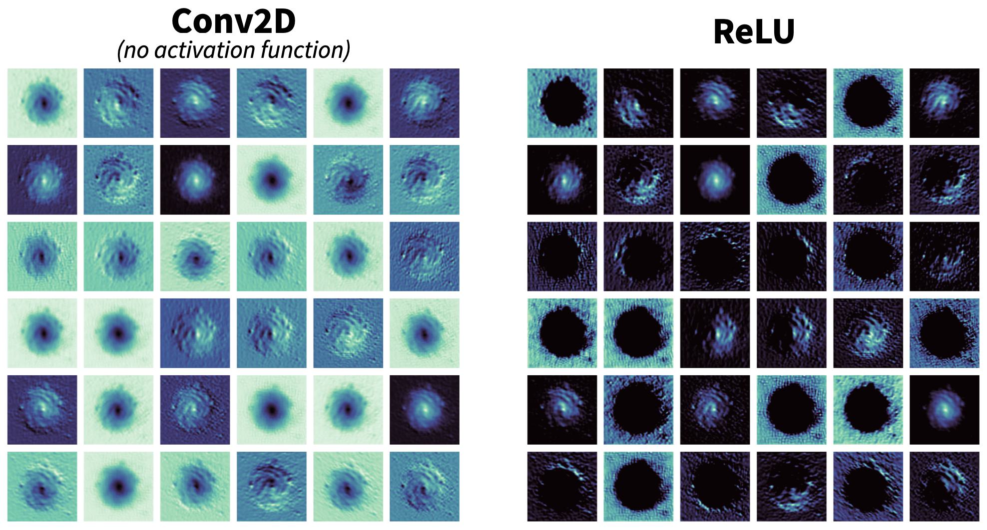
On the left we have the raw output of the Conv2D layer without any activation function. On the right is what we get when we process this raw output with the ReLU activation function. Immediately it’s clear that negative values have been eliminated; some feature maps now have holes where the galaxy used to be. Activation functions are important because they enforce nonlinearity. If we simply string together a series of convolutional layers without any activation functions, then our model will only ever be able to detect linear features (as the convolutions themselves are linear). In order for CNNs to effectively learn complex, abstract representations of arbitrary data, they simply must be able to detect non-linear features.
Pooling
Pooling layers are used to downsample feature maps. This is usually done with a 2×2 pool, hence resulting in outputs that are half the width/height of the input. There are two main types of pooling. Max pooling, used almost ubiquitously, preserves the largest value in the pool. The somewhat less common average pooling instead calculates the average value in the pool. Here’s a visual example of a 2D max pooling.
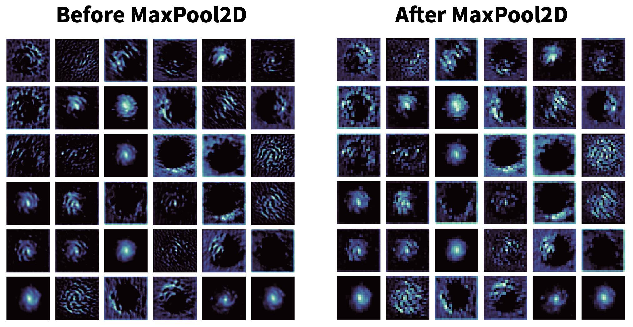
Pooling has the benefit of improving the robustness of the model, forcing it to focus on extracting more relevant features by learning more compact representations of the data. It’s also beneficial in terms of computation, with lower memory usage and less computational time.
Filter Weights
Recall from the introductory section that the convolutional filters are learnable; the filter weights are trained over time. Layer weights can be extracted in multiple ways:
# NB: get_weights() returns a list, we want the first element
weights = model.get_layer('conv2d').get_weights()[0]
weights = model.layers[i].get_weights()[0] # for some index i
Note that the shape of weights is (kernel_size, kernel_size, input_channels, output_channels), where kernel_size refers to the width of the convolutional filter/kernel. For example, suppose L1 is a convolutional layer that takes an RGB image input and outputs 32 feature maps, using a 5×5 kernel. This is followed by another convolutional layer, L2, which outputs 64 feature maps using a 3×3 kernel. Then weights has the shape (5, 5, 3, 32) for L1 and (3, 3, 32, 64) for L2. It’s worth normalising the weights before plotting, as well as converting to type uint8 especially if using matplotlib’s imshow or PIL/Pillow.
weights = (weights - np.min(weights)) / np.ptp(weights) * 255
weights = weights.astype('uint8') # important!
Below are some random, initial filter weights for L1, compared with the filter weights for L1 after being trained on the CIFAR-10 dataset. Notice how the colours are more subdued in the case of the trained weights.
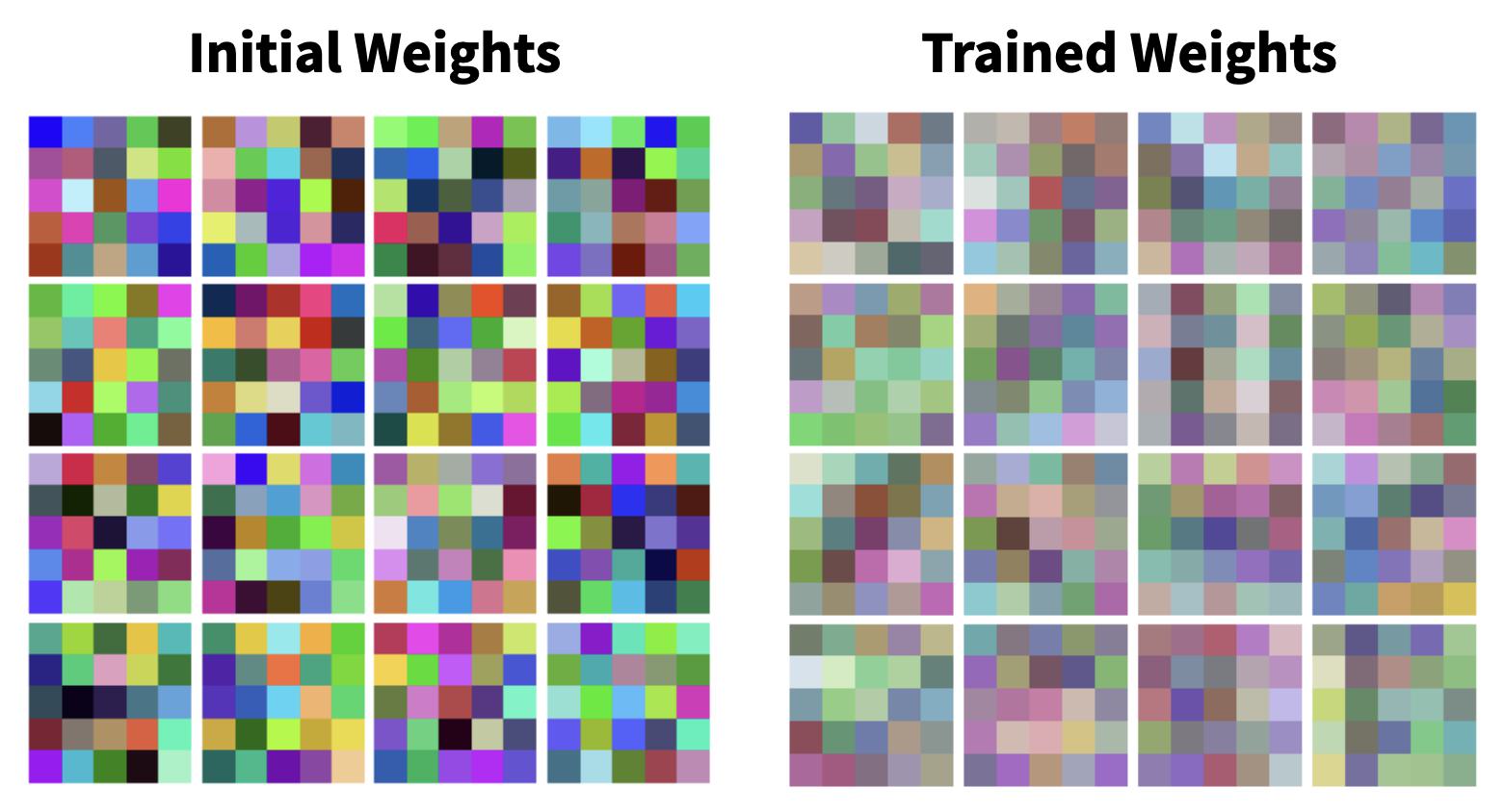
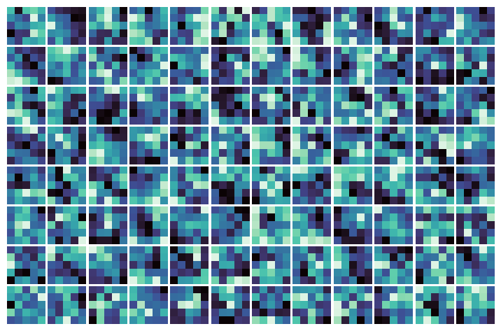
I should also note that it’s only possible to plot the filter weights of the first layer in colour (assuming your input image is also in colour!) since subsequent layers will undoubtedly have more than 3 input channels. Finally, here’s some filter weights for one of the layers of my galaxy CNN. Note the input is monochrome.
Filter Patterns
Convolutional filter weights on their own are not very interesting to look at; for the most part, they’re just noise, and it’s not clear what their purpose in life is. To that end, we can use a technique called gradient ascent to visualise the filter patterns. This technique is explored in detail in this excellent keras.io example by François Chollet. To be more precise, by “filter pattern” I mean
An input to the CNN that maximises the response of a specific filter (in a specific layer)
This is why we use gradient ascent, as we want to modify the image so that it more strongly activates the given filter. The overall gradient ascent approach can be roughly summarised as follows. To begin, we first provide a visually neutral, grey image as the input image. This is passed through the model to obtain the output activations at the desired layer. We then compute a loss value, which is simply the reduced mean of the activation for the given filter. We then compute the gradients of this loss with respect to the original input image, repeat these steps to iteratively update the image.
You can think of this technique as the “inverse” of training a network:
- When training a neural network, the weights are tweaked to minimised the loss (with respect to the training data) via gradient descent
- To visualise the filter patterns, we instead tweak an input image to maximise its activation (with respect to the filter weights) via gradient ascent.
Let’s go ahead and visualise each filter in each layer of my galaxy CNN.
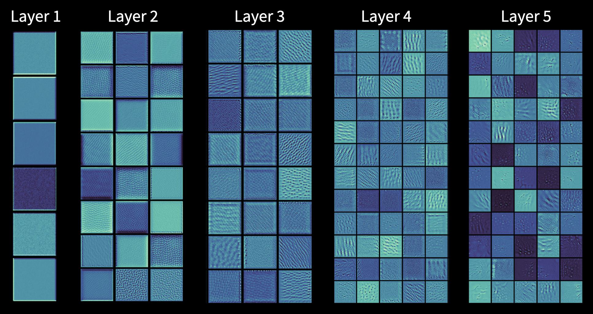
As we progress deeper inside the CNN, the filter patterns become richer and reveal more intricate detail, from wavy ripples to clusters of holes. This illustrates the clear benefits of having multiple convolutional layers.
Stripy patterns are very common filter patterns. Below are some example patterns for CNNs trained on the CIFAR-10 and Fashion-MNIST datasets:
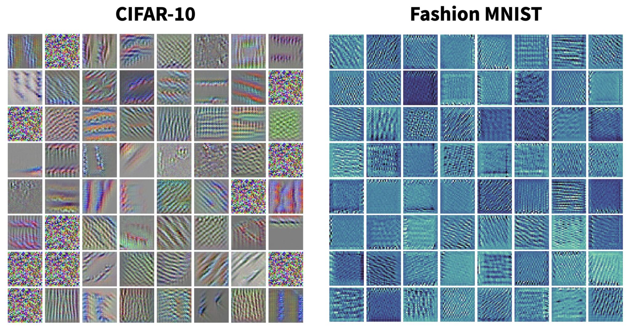
Note some filter patterns turn out to just be noise, in which case the filter isn’t responding to anything; this is more likely to occur in the first couple of layers of a network. For the actual gradient ascent process, we can compute a “pseudo-loss” – in terms of the activation with respect to the current filter – as follows:
# define a feature extractor as in the filter weight example
feature_extractor = keras.Model(inputs=model.input, outputs=model.get_layer('conv2d').output)
def get_loss(image, filter_index):
    # it's worth explicitly setting training=False, esp. if your model has preprocessing layers
    activation = feature_extractor(image, training=False)
    # trim borders of the feature map, the keras.io example uses 2:-2
    # but I find 1:-1 is better for deeper layers
    return tf.reduce_mean(activation[:,1:-1,1:-1,filter_index])
The core gradient ascent loop is essentially as follows:
for n in range(n_steps):
    with tf.GradientTape() as tape:
        tape.watch(image)
        loss = get_loss(image, filter_index)
    # calculate gradients of the "pseudo-loss" w.r.t the image
    gradients = tape.gradient(loss, image)
    # normalize the gradients, then update the image
    gradients = tf.math.l2_normalize(gradients)
    # it's useful to control the degree of change with a learning rate
    image += learning_rate*gradients
See the keras.io example for more.
Conclusion
Convolutional neural networks are incredibly powerful models capable of learning abstract representations of data through extracting meaningful features via the use of convolutional filters. Being able to visualise the outputs of convolutional layers, as well as visualising the patterns that the convolutional filters themselves are most responsive to, goes a long way in helping to understand how CNNs process data.
References & Further Reading
- Deep Learning with Python (2nd Edition) by François Chollet
- Keras code example: Visualizing what convnets learn (also by François Chollet)
- Feature Visualization, Distill.pub
- Stanford University’s CS231n publicly available course notes
- MIT’s 6.S192 Introduction to Deep Learning course notes and Youtube channel