The first deep-field image from the James Webb Space Telescope showcased the dazzling splendour of our distant Universe at an unprecedented resolution, with further follow-up images revealing an astonishingly diverse array of galaxy types. From ellipticals to spirals – and just about everything in-between – galaxies exhibit a remarkable range of structural forms and shapes collectively referred to as morphologies. Understanding the formation and evolutionary pathways of different morphologies is central to elucidating the physics that govern galaxies, as well as the physics that underpin our current cosmological models.
When it comes to galaxies, a key challenge lies in classifying their morphologies. This process is traditionally done by eye, often with a handful of expert astronomers – or large pools of volunteer citizen scientists – manually sifting through thousands upon thousands of galaxy images at a time. In recent years, deep learning techniques have made great strides to automate this process. Another more subtle challenge lies in categorising galaxy morphologies in the first place. After all, the terms “elliptical” and “spiral” stem from the eponymous classification system devised by Hubble in the 1920s, which defines morphology in terms of apparent visual appearance. While later refinements to this sequence have incorporated more galaxy subtypes, this inherently subjective definition of morphology remains a core point of contention. Some studies have gone so far as to use deep learning models to study the underlying structure of large datasets of galaxy images.
In my previous post on latent space visualisation, I discussed how deep learning models work by approximating data manifolds. In this post, I go a step further and explore the latent space of galaxy morphology using images from the Galaxy10 DECals dataset, a publicly-available dataset of high-resolution galaxy imagery included in the astronn package. To do this, I train several variational autoencoders to reduce the 17,736 galaxy images into points in lower-dimensional latent spaces. We will explore these latent manifolds, and see how their fundamental axes relate to galaxy morphology.
All models are coded in TensorFlow/Keras.
Autoencoders
Autoencoders are a family of unsupervised deep learning models designed to automatically learn some lower-dimensional representation of a given set of training data. This representation is also referred to as a code or encoding, but it is essentially a latent space. Autoencoders consist of two separate components:
- The encoder, which maps the input data to points in the latent space (a.k.a latent vectors)
- The decoder, which maps points from the latent space back into data.
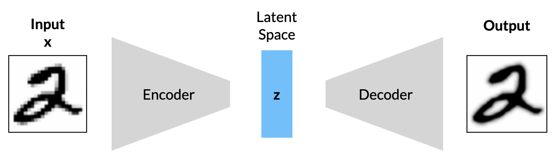
Both models are trained simultaneously, the goal being for the encoder to find the most efficient lower-dimensional encodings for the input, and for the decoder to reconstruct the input (based on the encodings) as closely as possible. Here, the latent space can be thought of as a forced information bottleneck. Autoencoders are essentially models with which to perform nonlinear principal component analysis (PCA), and are commonly used in applications involving dimensionality reduction and/or compression, similarity-based clustering, anomaly detection, and exploratory analysis. Autoencoders also have powerful applications in computer vision, such as image compression, image denoising, and even image colourisation.
As a quick example, let’s code a vanilla autoencoder and train it to classify images of handwritten digits from the MNIST dataset. In this particular example, both the encoder and decoder are components in the same Keras model (though we can easily separate them, as we will soon see). Here we use strided convolutions to process the input images, before flattening the outputs into the forced bottleneck (in this case a Dense layer with LATENT_DIM nodes). As the name implies, LATENT_DIM represents the dimensionality of the latent space. The output image is constructed with the use of strided transposed convolutions.
LATENT_DIM = 2
ae_in = layers.Input(shape=(28,28,1))
x = layers.Conv2D(32, 3, strides=2, padding='same', activation='relu')(ae_in)
x = layers.Conv2D(64, 3, strides=2, padding='same', activation='relu')(x)
x = layers.Flatten()(x)
x = layers.Dense(32, activation='relu')(x)
x = layers.Dense(LATENT_DIM, activation='relu', name='encout')(x)
x = layers.Dense(7*7*64,activation='relu', name='decin')(x)
x = layers.Reshape((7,7,64))(x)
x = layers.Conv2DTranspose(64, 3, strides=2, padding='same', activation='relu')(x)
x = layers.Conv2DTranspose(32, 3, strides=2, padding='same', activation='relu')(x)
ae_out = layers.Conv2D(1, 3, padding='same', activation='sigmoid')(x)
ae = keras.Model(ae_in, ae_out, name='autoencoder')

ae.compile(
    optimizer=keras.optimizers.Adam(learning_rate=1e-3),
    loss=keras.losses.BinaryCrossentropy()
)Now we can fit the model. This is one of those satisfying times when the input data \( x \) and target data \( y \) are the same!
ae.fit(images, images, epochs=50, batch_size=128)Once trained, we can “recover” the separate encoder and decoder parts of the autoencoder as follows:
encoder = keras.Model(ae.inputs, ae.get_layer('encout').output)
decoder = keras.Model(ae.get_layer('decin').input, ae.outputs)
Now we are free to obtain the latent space encodings from the inputs, and also to directly generate new images with the decoder.
# obtain encodings of the images in the latent space
z = encoder.predict(images)
# generate images from seeds
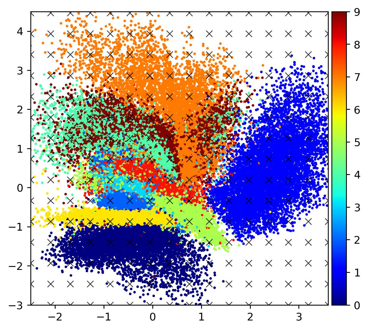
ex_images = decoder.predict(zsample)Let’s visualise the latent space. The scatter plot below shows the locations in the latent space of images in the MNIST dataset, coloured by their digit label. Although the autoencoder has managed to tightly cluster several digits, there is a significant amount of scatter and “empty space” between embeddings.
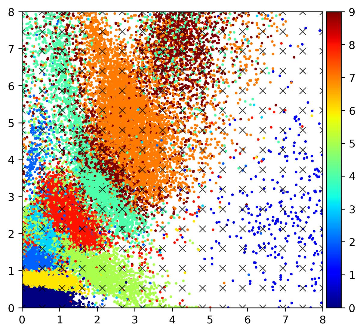
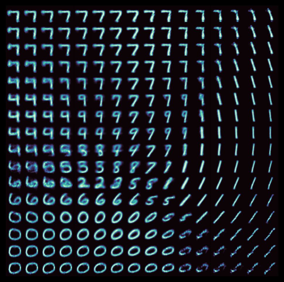
We can see the implications of the structure of the latent manifold when we try to generate a bunch of images with the decoder by sampling equally-spaced points on a grid. Each individual image below corresponds to an ‘X’ in the above scatter plot in its respective position.
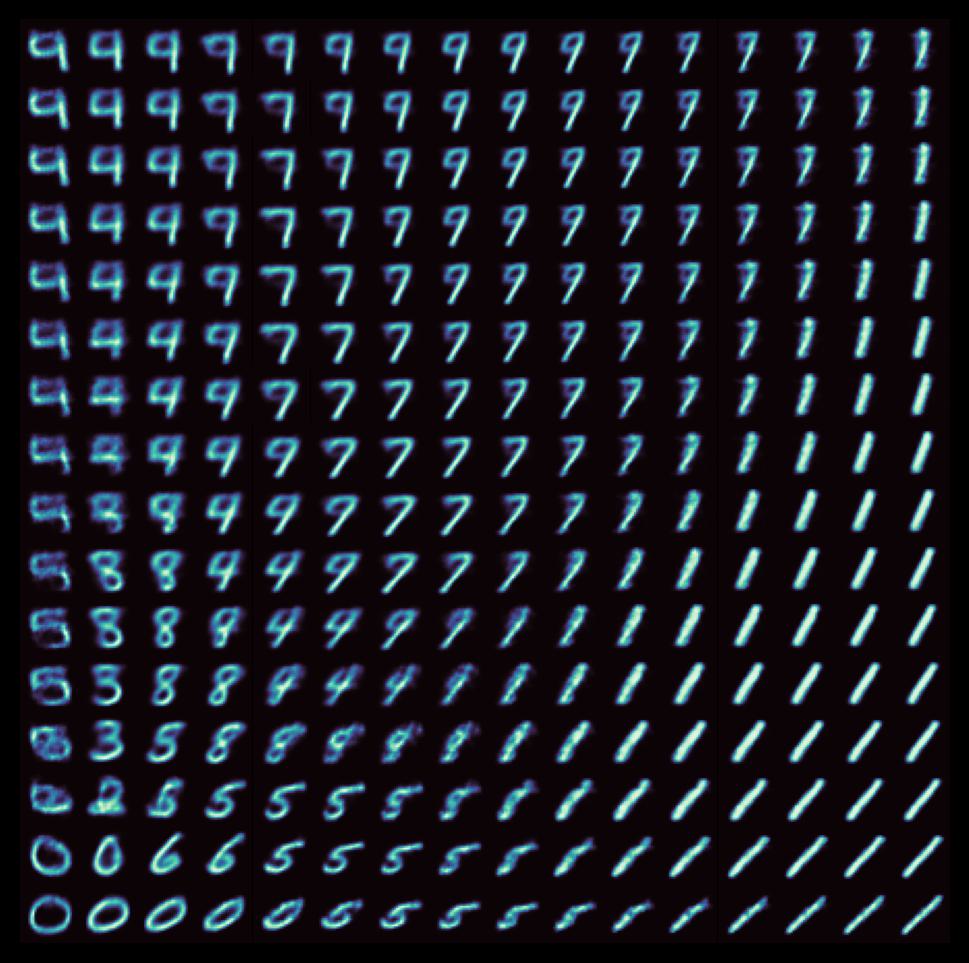
As can be seen, there are many points in the latent space which map to unrealistic digits, and it is difficult to interpolate along the manifold (consider traversing the first two columns, for instance). Indeed, one of the core issues with standard autoencoders is the discrete nature of the encodings; points are mapped directly to latent vectors. As such, data points tend to be clustered into largely disparate sets. This is fine – desirable, even – for applications involving clustering (as is the case with PCA and its contemporaries like t-SNE), but when it comes to using autoencoders to generate new datapoints, it’s better for the points on the latent space to be distributed more smoothly, so that one can better interpolate between points to generate novel data.
Variational Autoencoders
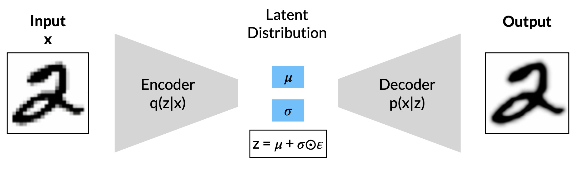
So, how can we map data into latents in such a way to generate new data more effectively? One deceptively powerful model takes the basic autoencoder architecture but instead utilises it within a probabilistic framework using techniques from variational inference. This model is the varational autoencoder or VAE. In a VAE, rather that mapping inputs to explicit points in a latent space, the encoder instead models data as parameters of a latent distribution (in particular, vectors of means and variances). Let’s reformulate the problem from this new probabilistic viewpoint in order to get some intuition behind the process.
Our input data constitute a set of examples taken from some high-dimensionality space \( x \). We want to represent this data in a latent space \( z \), where values \( z^{(i)} \) are drawn from some prior \( p_\theta(z) \). The role of the decoder is to generate new data points \( x^{(i)} \) using the conditional distribution \( p_\theta(x|z) \). Of course, in order to do that we need a way to map points from \( x \) into points in \( z \). Under ideal conditions, this can be easily modelled with the posterior: \[ p(z|x) = \frac{p(z)p(x|z)}{p(x)}\] Unfortunately, the true underlying posterior \( p_\theta(z|x) \) is generally intractable (by extension, so too is the marginal likelihood \(p(x)\) ). This is where the encoder comes in; we use it to model a new distribution \( q_\phi(z|x) \) with which to approximate the true posterior \( p_\theta(z|x) \). Note the use of \( \phi \) as a subscript to denote that the encoder uses a completely different set of parameters.
VAEs are trained by maximising what is known as the evidence lower bound (a.k.a variational lower bound). This is defined as follows: \[ L\left(\theta, \phi; x^{(i)}\right) = -D_{KL}\left(q_\phi(z|x^{(i)})||p_\theta(z)\right) \quad + \quad \mathbb{E}_{q_\phi(z|x^{(i)})}\left[ \log p_\theta (x^{(i)}|z)\right]\] Here the first term is the KL-divergence, which in this case is a statistical measure of how well the encoder \( q_\phi(z|x) \) approximates the true posterior \( p_\theta(z|x) \) using the prior \( p_\theta(z) \) as a proxy. The second term represents the cross-entropy, which in this case is a measure of the reconstruction loss; how well the decoder is able to generate new points \( x^{(i)} \) given \( z \).
The encoder \( q_\phi(z|x) \) is commonly modelled as a factorised Gaussian encoder where the means \( \mu \) and variances \( \log \sigma \) are direct outputs of the neural network. The final values \( z \) can then be sampled (from a univariate Gaussian distribution) as follows: \[ z = \mu + \sigma \odot \epsilon \] where \( \epsilon \sim N(0,\mathbf{I}) \) is just random noise. The inclusion of the auxiliary variable \( \epsilon \) is part of the reparametrisation trick, a reformulation that allows for the loss to properly backpropagate through the layers of the encoder. For a more thorough overview of VAEs, see Kingma & Welling (2019).
Below is a plot of a 2D latent space for the MNIST dataset using the same encoder/decoder CNN architectures, but this time trained together as part of a VAE (we’ll see this training in more detail in the next section).
The immediate difference is that the latent manifold is now considerably smoother, especially in the transition regions between different digits. Overall, the embeddings exhibit a far more appreciable global structure. This is a desirable property to have when investigating different galaxy morphologies in order to unearth some fundamental axes.
Galaxy Morphology with VAEs
To begin our exploration of the latent space of galaxy morphology, let’s first acquire and preprocess the Galaxy10 DECals Dataset. The raw images all have a resolution of 256×256, but in the interests of computational efficiency we will be downsizing these to 128×128. Let’s now craft some more powerful encoders and decoders to form the bedrock of our VAE. As before, these use strided convolutions.
keras.backend.clear_session()
LATENT_DIM = 2

encinp = layers.Input(shape=(128,128,3))
x = layers.Conv2D(32, 5, activation='relu', strides=2, padding='same')(encinp)
x = layers.Conv2D(64, 5, activation='relu', strides=2, padding='same')(x)
x = layers.Conv2D(128, 3, activation='relu', strides=2, padding='same')(x)
x = layers.Conv2D(192, 3, activation='relu', strides=2, padding='same')(x)
x = layers.Conv2D(256, 3, activation='relu', strides=2, padding='same')(x)
x = layers.Flatten()(x)
x = layers.Dense(256, activation='relu')(x)
z_mean = layers.Dense(LATENT_DIM, name='z_mean')(x)
z_log_var = layers.Dense(LATENT_DIM, name='z_log_var', kernel_initializer=keras.initializers.Zeros())(x)
z = VAESampling()([z_mean, z_log_var])
encoder = keras.Model(encinp, [z_mean, z_log_var, z], name='encoder')

decinp = layers.Input(shape=(LATENT_DIM,))
x = layers.Dense(4*4*256, activation='relu')(decinp)
x = layers.Reshape((4,4,256))(x)
x = layers.Conv2DTranspose(192, 3, activation='relu', strides=2, padding='same')(x)
x = layers.Conv2DTranspose(128, 3, activation='relu', strides=2, padding='same')(x)
x = layers.Conv2DTranspose(64, 3, activation='relu', strides=2, padding='same')(x)
x = layers.Conv2DTranspose(32, 5, activation='relu', strides=2, padding='same')(x)
decout = layers.Conv2DTranspose(3, 5, activation='sigmoid', strides=2, padding='same')(x)

decoder = keras.Model(decinp, decout, name='decoder')
Here the VAESampling layer is based on the official Keras VAE tutorial by François Chollet. Also note that the kernels for the the z_log_var dense layer are initialised to zero; I found that this helps to avoid issues with NaN losses after prolonged training. We will also use the same training code as per the tutorial. Unless otherwise specified, all VAEs are trained for 300 epochs with a batch size of 128.
Now then, let’s visualise the 2D latent space of our VAE. Here the dots are coloured based on their morphological label.
The overall manifold is primarily aligned in one direction, with some classes such as the edge-ons splayed outwards in a fan-like pattern. While classes such as round-smooth and in-between round-smooth are tightly clustered and well-defined, others such as disturbed and merging have very high degrees of scatter (though this is to be expected given their nature). As before, let’s sample some gridpoints and generate some galaxies with the decoder.
Here we can see that the splayed-out manifold is the VAE’s attempt to account for different orientations of edge-on and/or elongated galaxies. Looking at the two middle rows, the x-dimension appears to control for size, while the y-dimension controls for orientation and ellipticity. Of course, this is only what the manifold looks like with a 2-dimensional latent space; let’s now increase its size.
Comparing Latent Dimensionality
The series of plots below show new galaxy images created by the decoder (using a random, normally-distributed seed) for four independent VAEs with increasing latent space dimensionality.
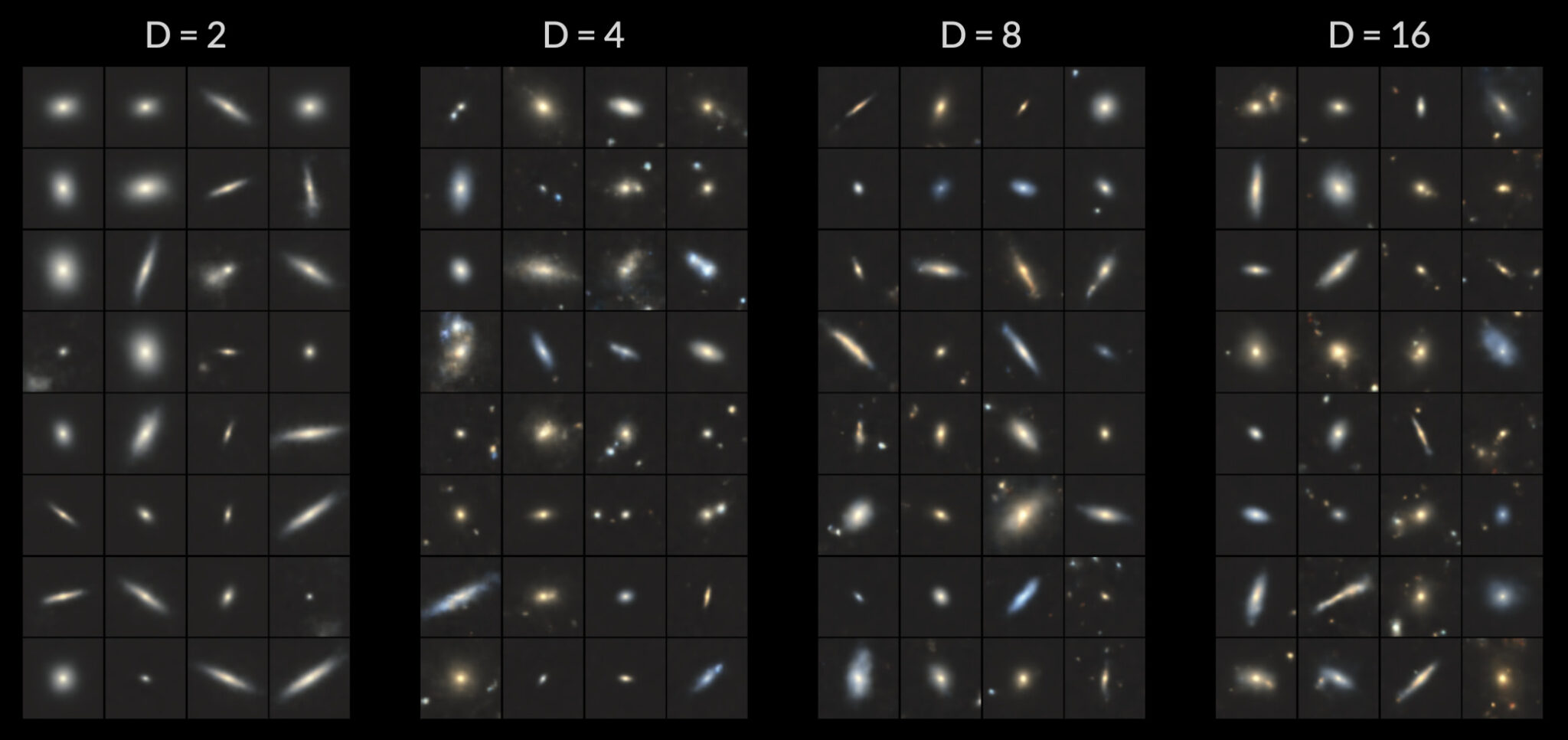
As we’ve seen in the 2-dimensional case, there is little to no information regarding colour; instead, samples differ only by shape. With 4-dimensions, we gain some semblance of colour, and the individual galaxies themselves are better defined. As we continue to double the dimensions of the latent space, the samples begin to look more and more realistic (albeit with diminishing returns). This should come as no surprise given that autoencoders essentially act as a means of data compression. It’s impressive that such a wide range of galaxy shapes with realistic colours can be generated from as few as four random numbers.
Four the 4-dimensional latent space, we’d need six 2D plots to visualise how each pair of dimensions interacts. Instead, let’s simply interpolate along each individual axis while keeping all the other axes set to zero.
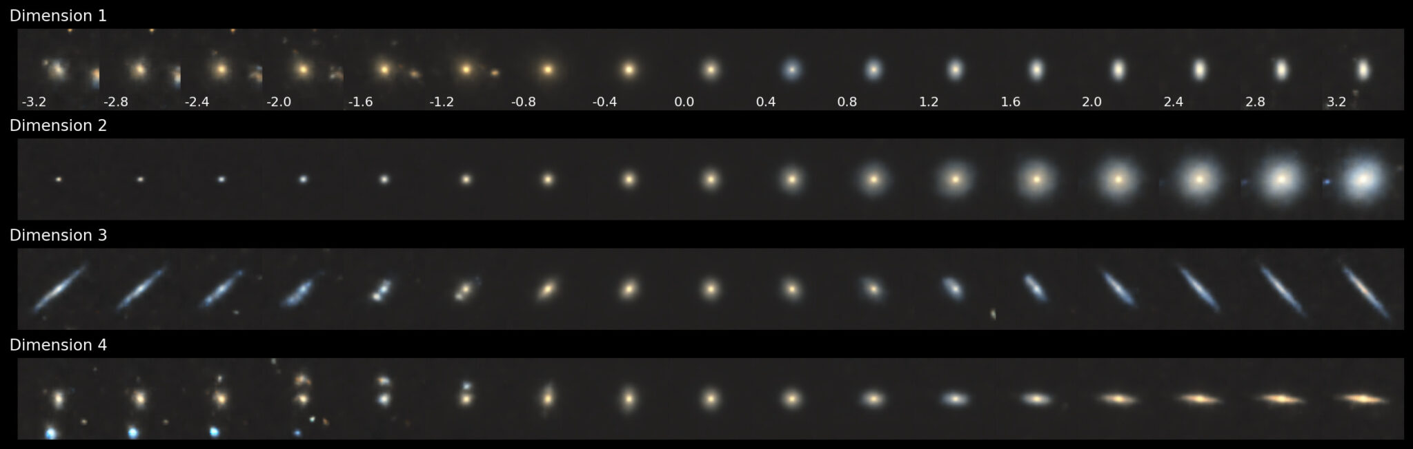
In this case, the 2nd dimension clearly controls for the size of the sample. The 1st dimension controls for colour while keeping the samples the same size. Dimensions 3 and 4 control for both colour and ellipticity. Now let’s see what this looks like for the 8-dimensional latent space.
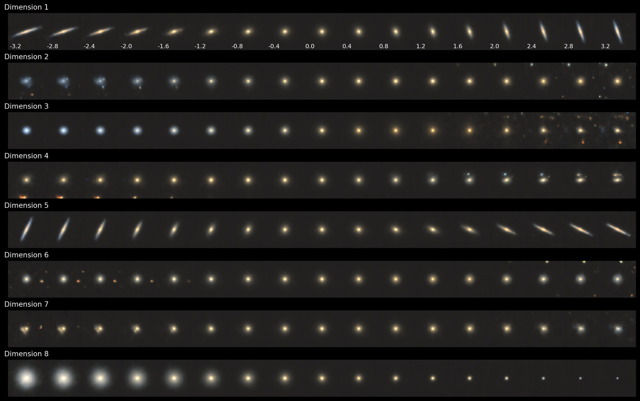
What’s amazing is that there is still only a single dimension that controls for size, namely Dimension 8 (near-identical to the reverse of Dimension 2 of the 4-D case). There are now two dimensions (1 and 5) that control for edge-ons in different orientations. Colour takes on more importance at this scale, as seen in Dimension 3. Furthermore, Dimension 2 shows the first clear signs of size-independent morphological transition, going from a blue irregular galaxy (negative values) to an elliptical galaxy (positive values). We also see the first hints of redundancies, with little distinction between the galaxies themselves in Dimensions 6 and 7.
Collapsing Dimensions
Perhaps we can get rid of these redundancies and further refine our latent spaces using some additional dimensionality reduction routines. Let’s take our 8-dimensional encodings from the VAE and reduce them to two dimensions using UMAP.
# here we are using the values for z_mean, see keras.io/examples/generative/vae
image_encodings, _, _ = encoder.predict(images)

# fit a UMAP model with the image encodings
mapper = umap.UMAP(n_neighbors=10, metric='euclidean', n_epochs=1000).fit(image_encodings)

# obtain the 2D embedding
embedding = mapper.transform(image_encodings)
We can plot the resulting 2D manifold as follows:
class_labels = ['Disturbed','Merging','Round Smooth','In-Between Round Smooth',
'Cigar Shaped Smooth','Barred Spiral','Unbarred Tight Spiral',
'Unbarred Loose Spiral','Edge-On w/o Bulge','Edge-On w/ Bulge']
fig = plt.figure(figsize=(9,7))
ax = fig.add_subplot(1,1,1)
sc = ax.scatter(embedding[:,0], embedding[:,1], cmap='jet', c=labels, s=1)
ax.legend(handles=sc.legend_elements()[0],
labels=class_labels, loc='lower center', ncol=3,
columnspacing=1, bbox_to_anchor=(0.5,0.99))
fig.colorbar(sc, ax=ax, pad=0)
ax.set_xlabel('z[0]')
ax.set_ylabel('z[1]')
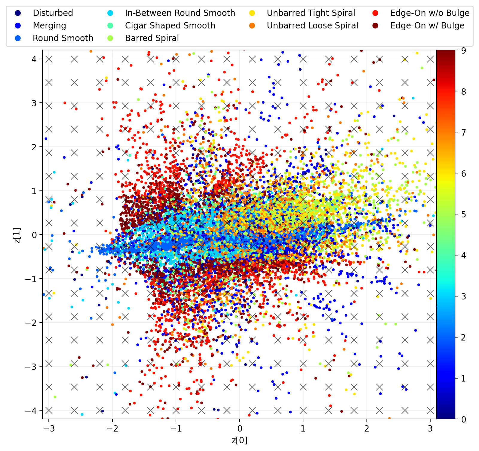
plt.show()Giving us the following plot.
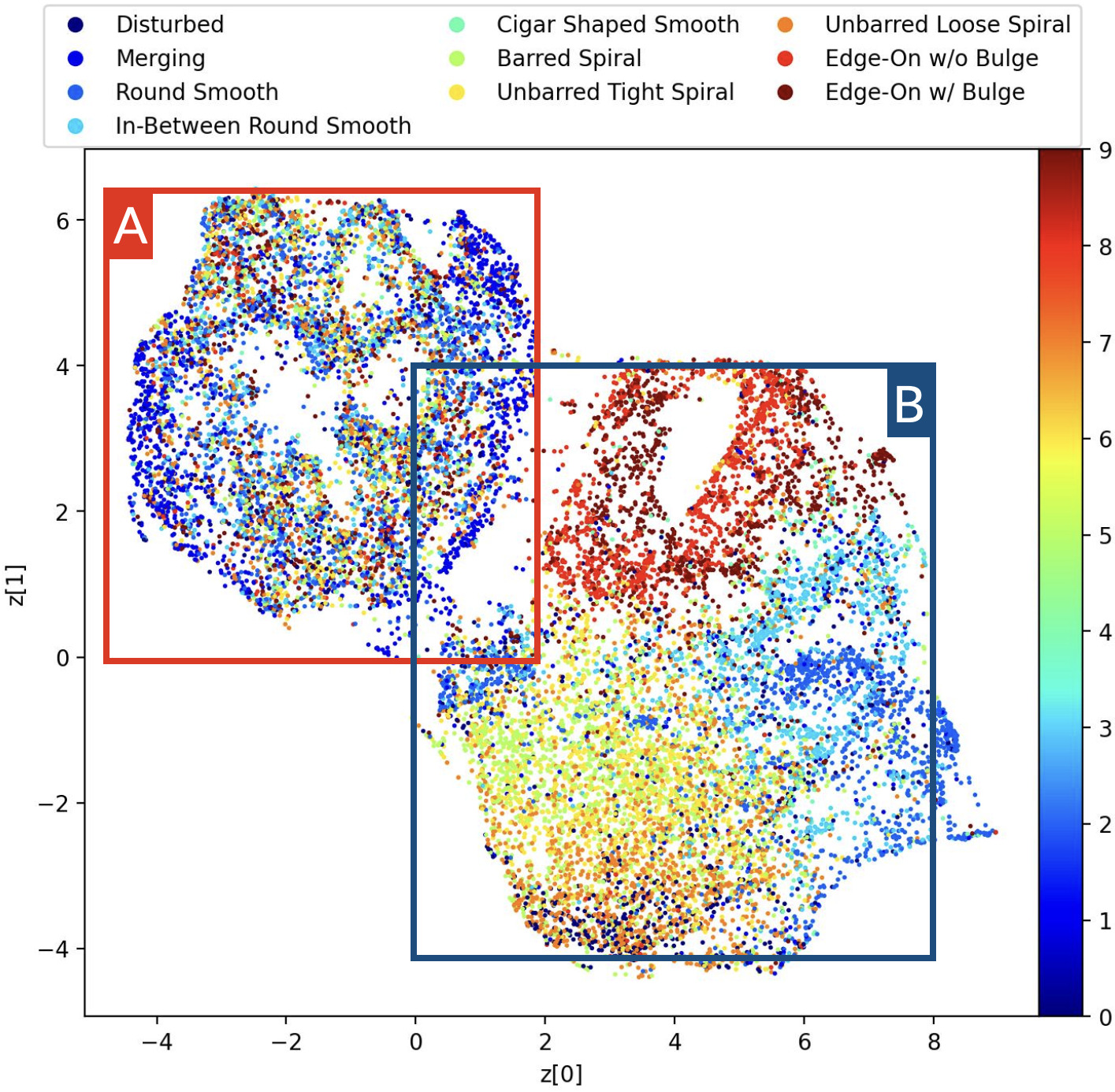
The embedding can be separated into two main groups. Group A contains a mix of morphologies, while group B is more cleanly separated with edge-ons at the top, spirals at the bottom-left and ellipticals mostly off to the right-hand side.
In order to generate galaxies at arbitrary points in the above scatter plot, we need a way to transform 2-dimensional points in the embedding into 8-dimensional points in the latent space of our VAE. Thankfully we can do this with UMAP’s inverse_transform:
seeds = mapper.inverse_transform(embedding_points)
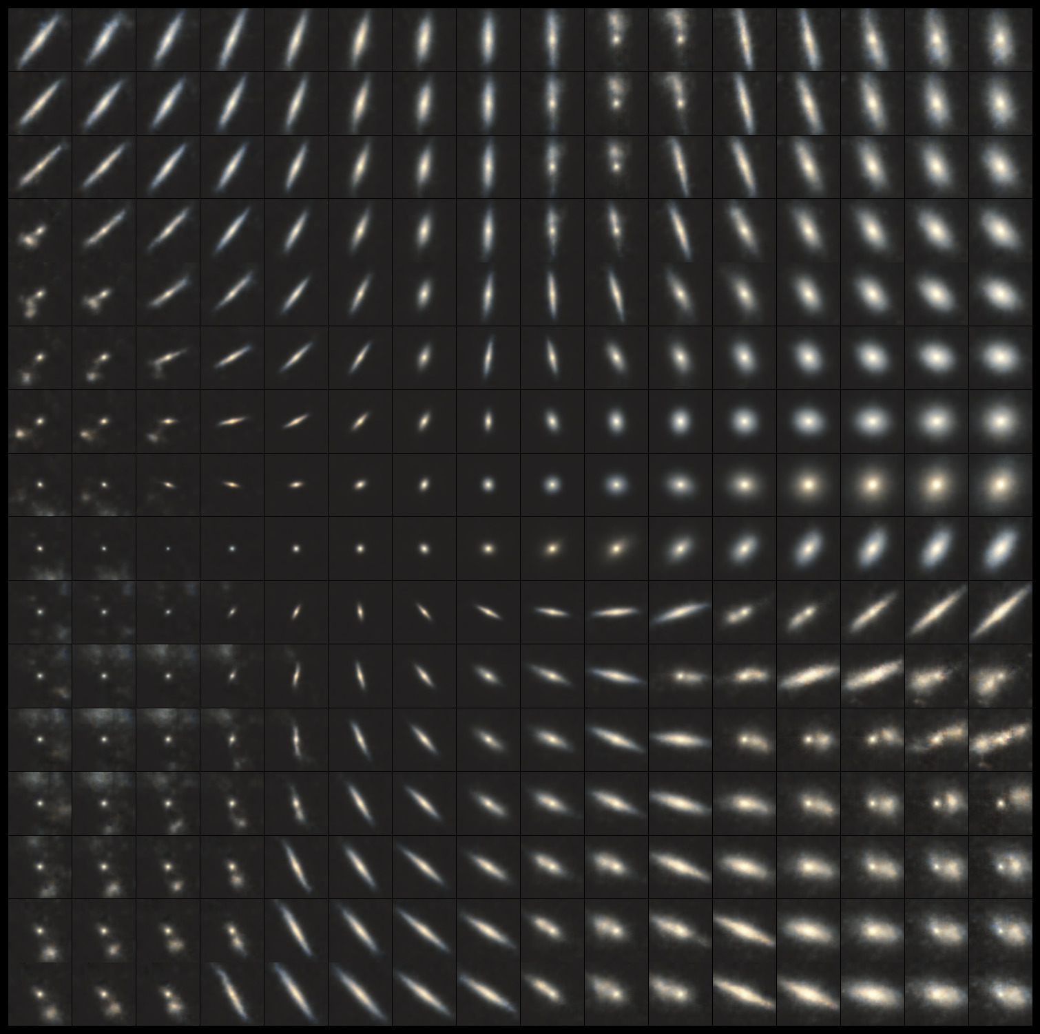
galaxies = decoder.predict(seeds, verbose=0)Having now obtained 8-dimensional seeds for each 2-dimensional point in the embedding, we can visualise the galaxies located within the Group A and Group B.
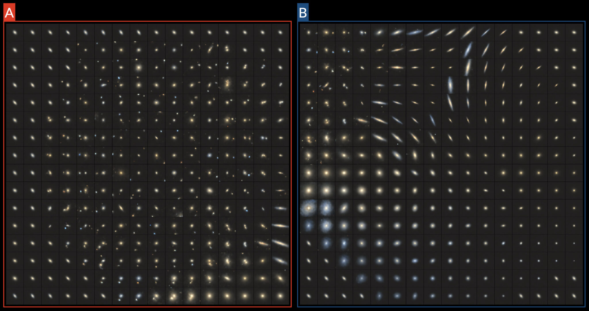
Interestingly, the galaxies located within the Group A manifold all contain foreground features, which appear to be radially arranged about the centre. As for Group B, as expected we find edge-on galaxies clustered at the top, with spirals (of varying colours) off to the bottom-left and ellipticals to the right.
Using UMAP allows us to further compress the latent space of a VAE. This can aid in interpretability (in that different classes can be more easily disentangled or grouped by similarity), but it’s important to keep in mind that this is merely a representation (same goes for the VAE encodings). Interpolation is more difficult due to the need to use an inverse transform to convert points in the embedding to points in the VAE’s latent space. So while UMAP is an excellent means for visualisation, it’s harder to determine exactly what each of the axes represents. Of course, this is a challenge inherent to any dimensionality reduction technique, but UMAP – and VAEs – allow us to uncover the underlying structure of arbitrary datasets, and explore patterns and features we otherwise would never see.
Summary
We have seen that variational autoencoders are powerful tools for nonlinear dimensionality reduction as well as for exploring and interpreting the latent spaces of arbitrary datasets. Their strength lies in their ability to approximate smooth, continuous manifolds that are well suited for interpolation. As such, VAEs make excellent generative models, however it’s worth noting that the images generated by VAEs tend to be somewhat blurry in comparison to other models such as generative adversarial networks.
In this post, we have used VAEs to analyse latent spaces of the Galaxy10 DECals dataset, which contains 17,736 galaxies grouped into ten morphological classes. In the direct 2-dimensional case, we’ve been able to reduce the dataset to one dimension for size, and another for orientation / ellipticity. With more dimensions, we can better account for colour and morphology. It’s possible to further disentangle the morphologies of galaxies by applying additional dimensionality reduction with UMAP to a higher-dimensional latent space.
Now it should be pointed out that this exploration of “morphology” is really only an exploration of the different morphologies encapsulated within the Galaxy10 DECals dataset. Of course, future high-resolution observational surveys will no doubt capture images of millions upon millions of galaxies. Perhaps at the heart of such a massive database of images lies a simple yet elegant latent space – a multidimensional Hubble Tuning fork capable of accounting for every galaxy morphology imaginable. That would certainly make classifying them a heck of a lot easier!