Galaxies have a remarkably versatile range of shapes and sizes, from majestic spirals to clumpy irregulars to Mexican hats and just about everything else in between. The inherent structural characteristics of a galaxy is referred to as its morphology. Categorising galaxies into their respective morphological classes might seem like nothing more than mere stamp collecting, yet it’s a necessary first step to understanding (and validating) the physical models that underpin both galaxy evolution and the larger-scale cosmological evolution of the Universe.
Modern morphological classification is still heavily derived from Hubble’s classification schema originally devised in the early 1900s: the affectionately-named Hubble Tuning Fork. Such schema are primarily based on the subjective visual inspection of a galaxy’s qualitative appearance and features (spiral arms, bulges, bars, etc.), though newer schemas also consider quantifiable, measurable properties like star formation rates.
Is it possible to characterise morphology based solely on an unsupervised model that can approximate the underlying, latent structure of a large dataset of galaxy images? Studies have explored this idea well before the advent of generative deep learning, applying models such as self-organising maps.
In a previous post, we trained a variational autoencoder (VAE) on the Galaxy10 DECaLS dataset (publicly available via the astronn python package) and created a “morphological atlas” via latent space exploration. In this post, we’ll revisit exploring the latent space of galaxy morphology, but this time with a Vector-Quantized VAE (VQ-VAE) paired with an autoregressive conditional transformer prior (this is essentially 2 out of 3 components of the original DALL-E image model; everything except CLIP). To make our prior more flexible, we can train it with class dropout to allow it to make conditional and unconditional predictions, allowing us to do CFG-style inference a là Stable Diffusion.
Before we get started, let’s briefly recap what an autoencoder is.
Autoencoders and VAEs
An autoencoder is a type of deep learning model with two distinct components:
- An encoder, which takes some input data \(x\) and compresses it into some vector \(z\) in a lower-dimensional latent space.
- A decoder, which takes the low-dimensional latent vector \(z\) and reconstructs the original input \(x\).
The usual metaphor here is data compression; the autoencoder is trained to find some efficient (lower-dimensional) latent representation of the input data. It’s important to note that autoencoders do not strictly have to “reconstruct” the input data \(x\); you can just as easily use them to map the inputs \(x\) into some target output \(x’\). Examples of this include image denoising and colour restoration.
Variational autoencoders are a type of generative deep learning model with several notable differences to regular autoencoders that make them more suitable for generating new data. Instead of transforming \(x\) into a latent vector \(z\), the encoder instead transforms \(x\) into the parameters of a (probabilistic) latent distribution, which is usually a (multivariate) Gaussian prior defined by \(z_{\mu}\) and \(\log z_{\sigma}\). The decoder then samples a new latent vector \(z\) from this distribution, and uses that to reconstruct the output. Once trained, we can sample from this probability distribution to synthesise new data samples. The role of the encoder has changed from simply finding an efficient encoding to approximating the true posterior of our input data. For more on this, check out the original paper.
Since the latent space is a continuous probability distribution, VAEs are well-suited for downstream exploratory analysis and manifold learning tasks (such as PCA / t-SNE), and it is relatively easy to visualise how inputs change as you navigate through the latent space. It is also very easy to make new images: simply sample from the probability distribution. However, images generated by VAEs tend to be execessively smooth, and it is near-impossible to get VAEs to reproduce high-level features to the same fidelity as generative adversarial networks (GANs).
So, how can we tweak the standard VAE formula to give the model the expressive power it needs to generate more realistic images, while preserving an highly interpretable latent space (something difficult to achieve with GANs). Turns out we just need to add a third model component to the mix: a vector quantizer.
Vector Quantization
The core aim of vector quantization is to transform some continuous data distribution into a discrete categorical distribution. We can do this choosing a set of “codebook” vectors, then mapping all points in the data distribution to the closest codebook vector. This process is essentially a type of Voronoi partition with the codebook vectors as centroids, and where the goal is to arrive at a set of codebook vectors that best represents the original distribution. It’s worth visualising this with a simple 2D example:
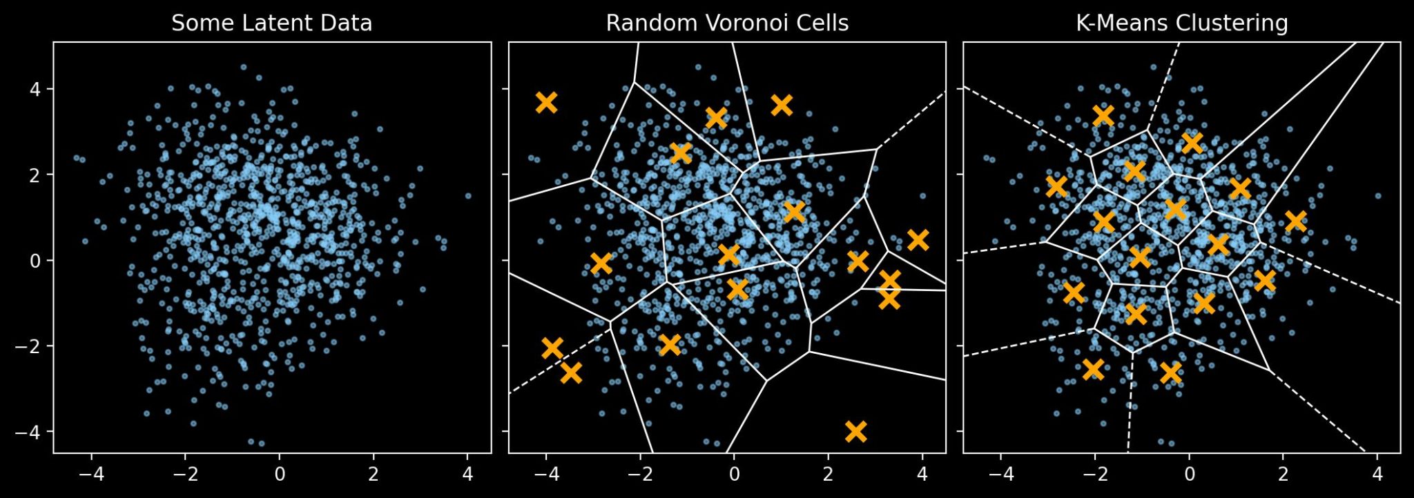
For this example we have some randomly distributed data created with scikit-learn’s make_blobs. The central panel shows a set of randomly-chosen points and their Voronoi tesselation. The right panel shows a different Voronoi tesselation, this time with points chosen via the K-means clustering algorithm (not to be confused with the k-nearest neighbour algorithm). Here the region is partitioned into Voronoi cells such that each data point belongs to the cell with the closest mean, and that the variance of points within each cluster is minimised.
VQ-VAE Components
Perhaps you can see where we are going with this. In a VQ-VAE, we use a vector quantizer with a learnable codebook. In other words, it’s up to the model to decide what codebook vectors to use in order to best represent the underlying data distribution and reveal the most meaningful latent components.
The core VQ-VAE architecture thus comprises three elements:
- An encoder, which behaves like a typical VAE encoder, transforming the inputs \(x\) into latent vectors \(z_e\).
- A vector quantizer, which takes these latent vectors \(z_e\) and maps vector to the nearest codebook vector in its learnable codebook. It returns both these codebook vectors \(z_c\) and the associated codebook indices \(i_c\).
- A decoder, which behaves like a typical VAE decoder, transforming the codebook vectors \(z_c\) into the target outputs \(x\).
It’s important to return the codebook indices \(i_c\) so that we know how to sample from the codebook to generate new data. More on that later.
Training a VQ-VAE on Galaxy10 DECaLS
The Galaxy10 DECaLS dataset contains 17,736 images of galaxies grouped into 10 morphogical categories. From 0 to 9, these are “disturbed”, “merging”, “round smooth”, “in-between round smooth”, “cigar shaped smooth”, “barred spiral”, “unbarred tight spiral”, “unbarred loose spiral”, “edge-on without bulge” and “edge-on with bulge”.
In this post we use images downsampled from the original 256×256 pixel size to a size of 128×128. Also, since my last ML blog posts, I’ve firmly switched from Keras/TensorFlow to PyTorch.
Encoder
For our encoder and decoder, let’s go with a typical sequential CNN structure with batch normalization and ReLU activation. The encoder maps tensors of shape (B, 3, 128, 128) to (B, embedding_dim, 16, 16):
encoder = nn.Sequential(
    nn.Conv2d(3, 32, kernel_size=3, stride=2, padding=1),  # (B, 32, 64, 64)
    nn.BatchNorm2d(32),
    nn.ReLU(),
    nn.Conv2d(32, 64, kernel_size=3, stride=2, padding=1),  # (B, 64, 32, 32)
    nn.BatchNorm2d(16, 64),
    nn.ReLU(),
    nn.Conv2d(64, 128, kernel_size=3, stride=2, padding=1),  # (B, 128, 16, 16)
    nn.BatchNorm2d(32, 128),
    nn.ReLU(),
    nn.Conv2d(128, embedding_dim, kernel_size=3, stride=1, padding=1),
)
Decoder
The decoder, of course, goes back the way it came, mapping tensors of shape (B, embedding_dim, 16, 16) back to (B, 3, 128, 128):
decoder = nn.Sequential(
    nn.Conv2d(embedding_dim, 128, kernel_size=3, stride=1, padding=1),  # (B, 128, 16, 16)
    nn.BatchNorm2d(128),
    nn.ReLU(),
    nn.UpsamplingNearest2d(scale_factor=2),
    nn.Conv2d(128, 64, kernel_size=3, stride=1, padding=1)  # (B, 64, 32, 32)
    nn.BatchNorm2d(64),
    nn.ReLU(),
    nn.UpsamplingNearest2d(scale_factor=2),
    nn.Conv2d(64, 32, kernel_size=3, stride=1, padding=1)  # (B, 32, 64, 64)
    nn.BatchNorm2d(32),
    nn.ReLU(),
    nn.UpsamplingNearest2d(scale_factor=2),
    nn.Conv2d(32, 3, kernel_size=3, stride=1, padding=1),  # (B, 3, 128, 128)
    nn.Tanh(),
)
Here we’ve used explicit upsampling layers to avoid the checkerboarding you normally see with ConvTranpose2d. Also note this uses Tanh as the final activation, so the images in the training data ought to be rescaled to [-1, 1].
The latent space in this example has a width and height of 16, for a total size of 256. This will be very important later.
A Simple VectorQuantize Example
For this post I will use the excellent VectorQuantize class from lucidrains/vector-quantize-pytorch. That said, it’s worth illustrating a very simple, stripped-down example to show how the data is being transformed. For this we’ll stick with just three parameters: the dimensionality of the input sequence (i.e. embedding dimensions); the number of vectors in the codebook (i.e. the codebook size); and the commitment beta, which is used in the loss calculation.
The codebook is just any old nn.Embedding layer:
class VectorQuantizer(nn.Module):
    def __init__(
        self, dim: int, codebook_size: int, commitment_beta: float = 0.25
    ) -> None:
        self.dim = dim
        self.codebook_size = codebook_size
        self.commitment_beta = commitment_beta
        self.embedding = nn.Embedding(codebook_size, dim)
        nn.init.uniform_(
            self.embedding.weight, -1.0 / codebook_size, 1.0 / codebook_size
        )
The forward pass proceeds as follows. First, we flatten the tensor and determine its nearest neighbours to the codebook vectors (which are the weights of the embedding layer). Here the input tensor has the shape (B, N, C) where B is the batch dimension and N is the sequence length for compatibility with vector-quantize-pytorch.
b, n, c = z.shape
assert c == self.dim
z_flat = z.reshape(-1, self.dim)
dists = torch.cdist(z_flat, self.embedding.weight, p=2.0) ** 2
indices = torch.argmin(dists, dim=1)
Now we quantize the original tensor z by selecting the nearest codebook vectors as specified by the original indices:
z_quantized = self.embedding(indices).view(b, n, c)
indices = indices.view(b, n)
The total loss involves two separate terms; the codebook loss and commitment loss. The commitment_beta hyperparameter is a weight term for the commitment loss. Notice the shift in gradient assignment.
# Move the codebook vectors closer to inputs
codebook_loss = F.mse_loss(z_quantized, z.detach())

# Move the inputs closer to codebook vectors
commitment_loss = F.mse_loss(z_quantized.detach(), z)

loss = codebook_loss + self.commitment_beta * commitment_loss
We’re not quite there yet as z_quantized is actually missing its own gradients. Since z_quantized is discrete, we cannot directly differentiate it, but we still need to provide a gradient for backpropagation. One way to do this is to just pass through the gradient of the original tensor z. This method is, aptly, called the straight-through estimator.
z_quantized = z + (z_quantized - z).detach()And that’s it! We can return z_quantized, indices and the total loss for training.
The VQ-VAE Module
We can wrap all three components into a dedicated VQVAE module.
class VQVAE(nn.Module):
    """General-purpose VQ-VAE module for use with vector-quantize-pytorch"""

    def __init__(self, encoder: nn.Module, decoder: nn.Module, vq: nn.Module) -> None:
        super().__init__()
        self.encoder = encoder
        self.decoder = decoder
        self.vq = vq

    def forward(
        self, x: torch.Tensor
    ) -> tuple[torch.Tensor, torch.Tensor, torch.Tensor]:
        z = self.encoder(x)

        h, w = z.shape[-2:]
        z = rearrange(z, "b c h w -> b (h w) c", h=h, w=w)
        z_quantized, indices, loss = self.vq(z)
        z_quantized = rearrange(z_quantized, "b (h w) c -> b c h w", h=h, w=w)

        x_recon = self.decoder(z_quantized)
        return x_recon, indices, loss
Note since our inputs are images, \(x\) has the shape (B, C, H, W), and so we need to reshape it to the expected vq input shape of (batch, seq_len, dim). Similarly, z_quantized needs to be reshaped back into an image. We can infer the height and width of the latent space based on the encoder output shape.
For simplicity when training, we can define our loss function as the sum of the VectorQuantize loss and the reconstruction loss:
x_recon, indices, commit_loss = vqvae(x)
recon_loss = loss_fn(x_recon, x)
total_loss = recon_loss + commit_loss
This can slot right into a typical single-model, single-optimizer loop, such as with PyTorch Lightning (or Lightning Fabric for minimalism).
For the primary model that I will use throughout the rest of this post, I used the standard VectorQuantize module from vector-quantize-pytorch changing only the following settings:
dimof 256 (embedding dimensionality)codebook_sizeof 1024
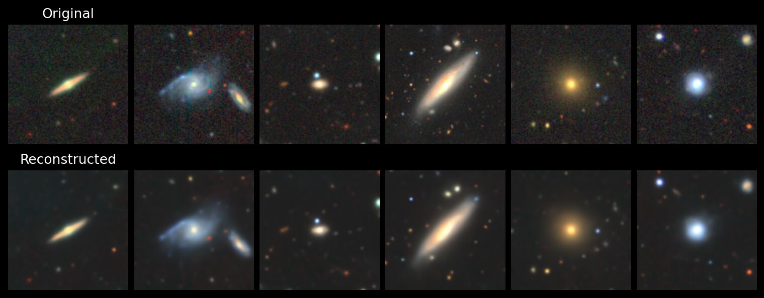
After ~500 or so epochs you should get something that looks like this:
Dimensions and Sizes
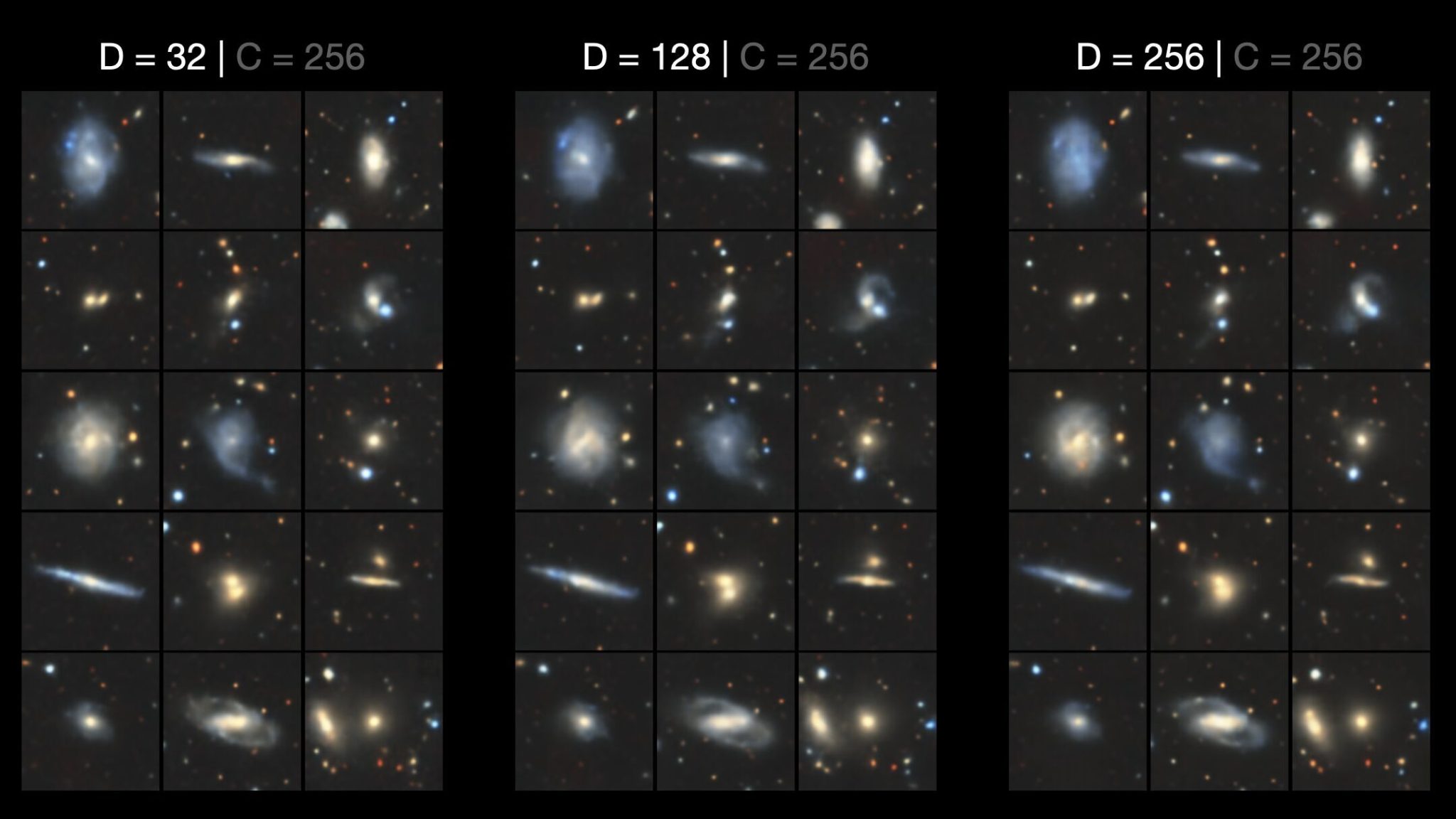
The question “how well did we do” naturally leads to “what if we changed X”. In particular, which parameter has the biggest impact on image quality: embedding dimensionality or codebook size? First, let’s compare the reconstructed images for VQ-VAEs with different embedding dimensionalities:
Now let’s see the impact of different codebook sizes:
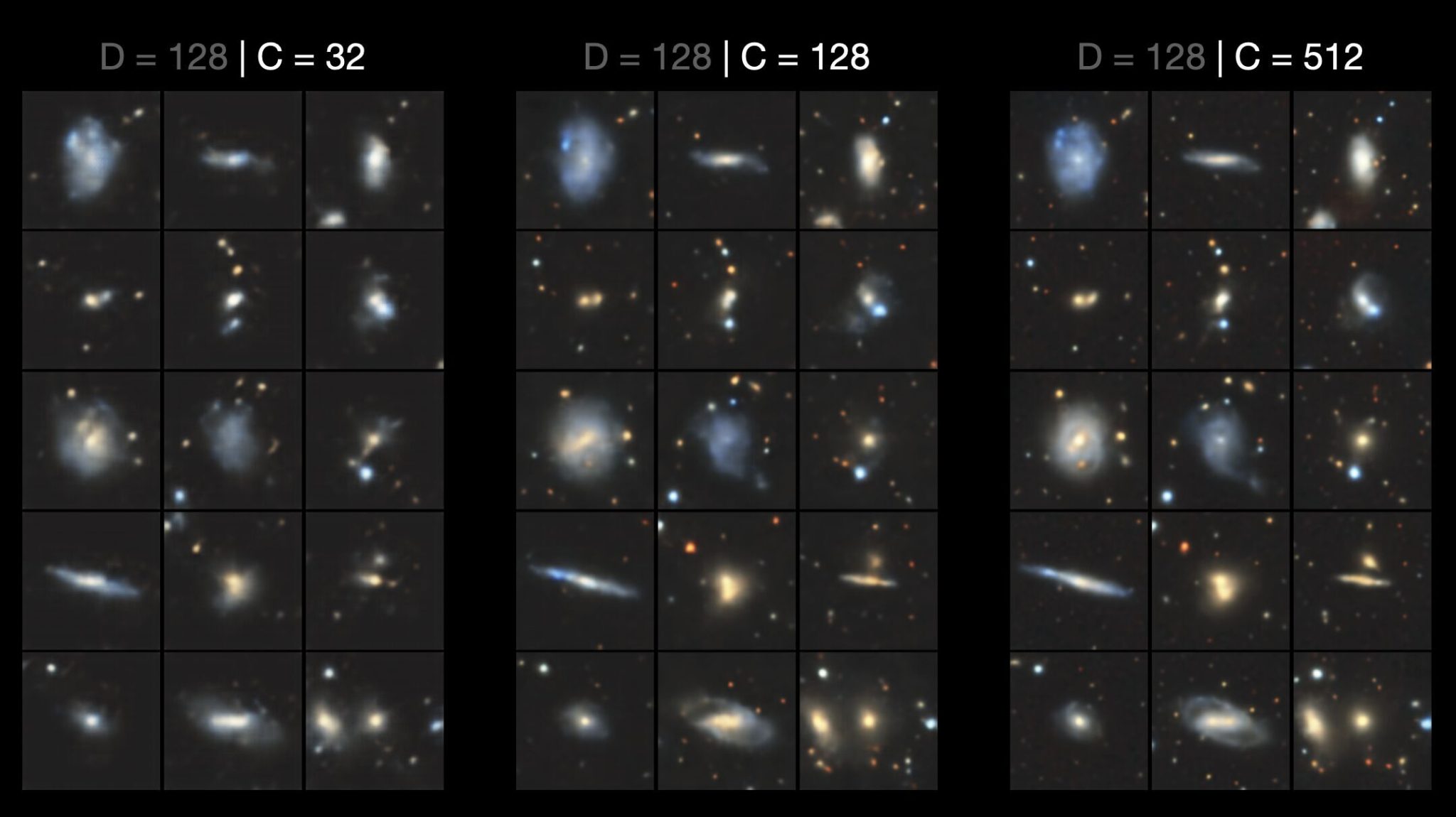
It’s quite the difference. For a fixed codebook size, changing the embedding dimensionality had relatively little impact, even for values as low as 32. Conversely, changing the codebook size has a dramatic effect on image quality. At low codebook sizes the colours appear more washed out and the galaxies themselves appear blurry. While for larger codebook sizes, the images are sharper with more high-level features.
To understand why changing the codebook size has such a big impact on the fidelity of the reconstructions, it’s high time we explored the VQ-VAE codebook.
Code Frequencies
A good place to start is examining the codebook utilisation, i.e. the percentage of codes that are actually indexed with the vector quantizer. This is the quickest way to spot codebook collapse. We can visualise with with a histogram and cumulative density function:
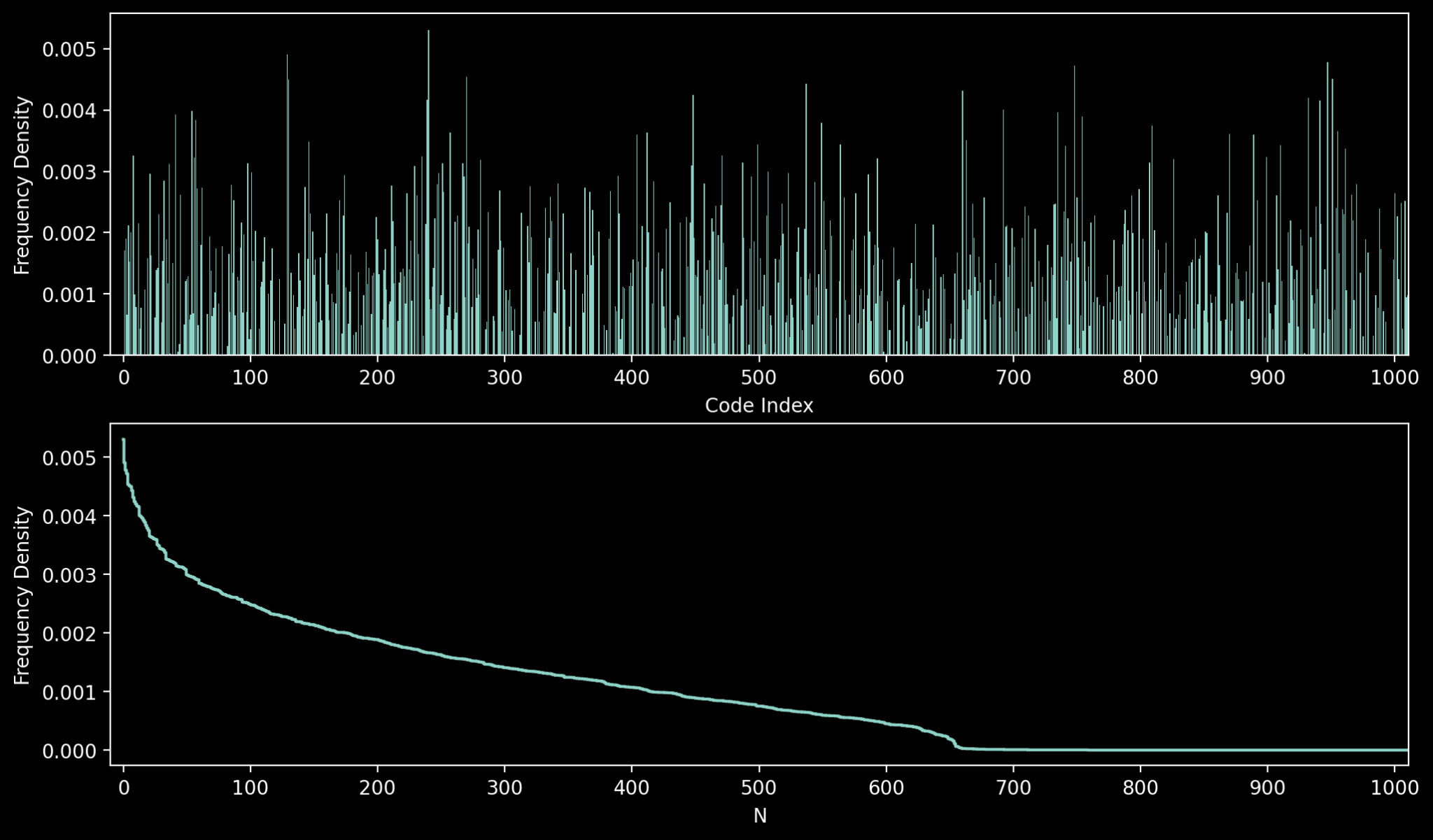
We can see that the codes extend throughout the full range of indices, but the counts are clearly non-uniform. There’s a sharp drop in frequency for the top 50 or so codes, yielding to a long tail that eventually collapses to 0. Indeed, for this particular model, the total codebook utilisation turns out to be around 66%; that is, around a third of the codebook vectors are never selected. This unused capacity shows that we still have room to improve, but it is nevertheless a good result. Codebook collapse is a failure mode where the vector quantizer only ever uses an extremely small selection of codebook vectors (usually in the single digit % range). Like the similar phenomenon of mode collapse in GANs (where the generator produces the same image), it’s a form of representation failure.
The codebook utilisation percentage is far from the only metric we can use to measure the efficiency of the codebook, and if anything it’s not the most reliable since the frequencies of each code are radically different. A more natural metric is perplexity, which gives us a better measure of how evenly the codes are utilised. Perplexity is the exponential of the information entropy (a.k.a Shannon entropy). We can calculate it for our indices as follows:
index_counts = torch.bincount(indices.flatten(), minlength=CODEBOOK_SIZE)
p = index_counts.float() / index_counts.sum()  # convert to probabilities
epsilon = 1e-10  # to avoid log(0)
entropy = -torch.sum(p * torch.log(p + epsilon))
perplexity = torch.exp(entropy)
If the codebook only ever uses a single code, then the entropy is 0 and the perplexity is 1. If all codes are equally likely to be used, then entropy is maximised and the perplexity equals the number of codes. In our case the perplexity of our model is 544, which implies an effective codebook usage of ~53%. This is well below the raw utilisation percentage of 66% of codes that have been used at least once, which implies the distribution of codes is non-uniform, as we saw in the previous figure. Ideally, perplexity should not to be too high or too low. Low perplexity is a sign of overfitting, while very high perplexities is a sign that the model is failing to train properly (as it’s effectively picking codes at random).
Heads and Tails
Since the frequency counts are dominated by a relatively small number of codes, what images does the VQ-VAE decoder produce when we feed it an input sampled from only these Top N codebook vectors?
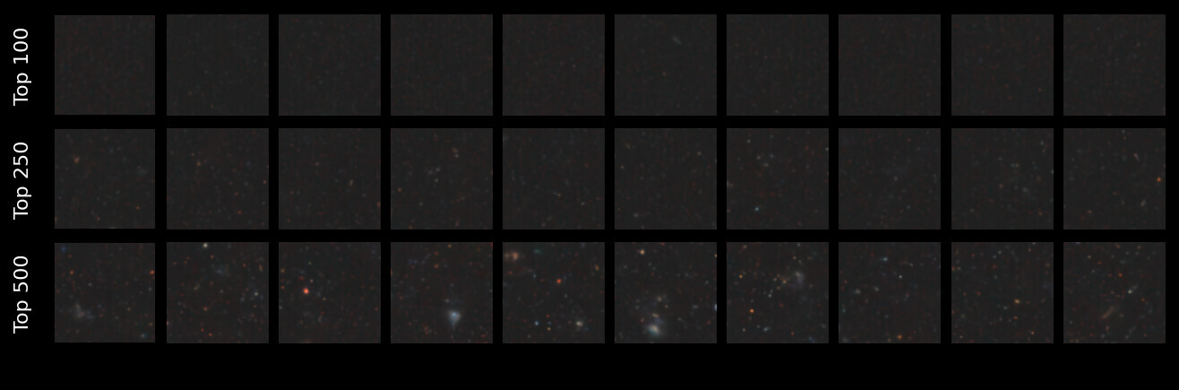
An image of a galaxy is, after all, dominated with a dark background, so it makes sense that the most common codes produce nothing but empty space and diffuse smudges. Only when we gradually incorporate more codes do we start to see higher-level details like stars.
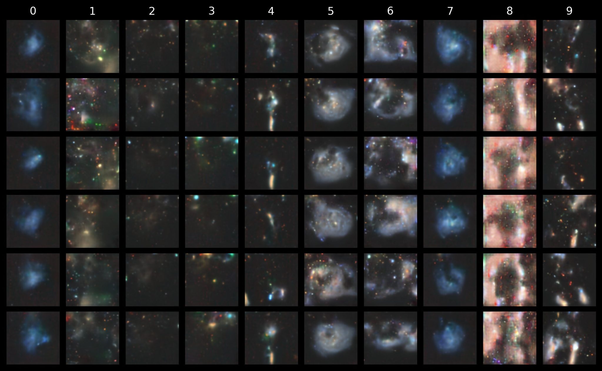
So, what happens when we generate images using only the Bottom N codes (excluding the unused codes, of course).
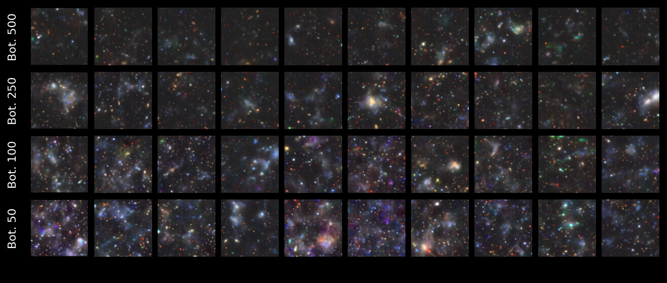
Turns out it’s the rare codes that actually represent the high-frequency structural components of the foreground galaxies. This might seem counterintuitive (especially to an astronomer), but this is true of the inherent statistics of any database of images: most of the pixels correspond to smooth regions, while only a few pixels occupy the crucial edges and textures that (to our eyes) make up the meaning of the image. The codebook utilisation frequencies are a power law because the latent pixel space of an image is itself a power law.
Just for fun, what happens when we give the VQ-VAE decoder an input composed entirely of (randomly selected) unused codebook vectors?
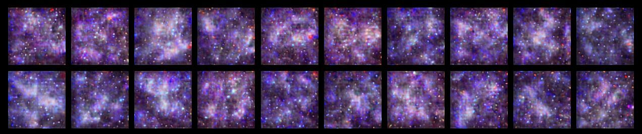
It’s not that surprising to see such an amalgamation since the unused codes are inputs the VQ-VAE decoder has never seen; the model has to interpolate in order to make sense of them.
Individual Codes
We’ve looked at codes as a collective but are yet to inspect what each individual code actually looks like. To actually retrieve the codebook vector for a given index, we need to sample the codebook embedding. Luckily the VectorQuantize model has a handy get_codes_from_indices to do just that.
with torch.inference_mode():
    indices = torch.full((256,), index, dtype=torch.long, device=device).unsqueeze(0)  # shape = (b, h * w)
    z_quantized = vq.get_codes_from_indices(indices)  # shape = (b, h * w, c)
    z_quantized = z_quantized(code_vector, "b (h w) c -> b c h w", h=16, w=16)  # i.e. reshape
    gen_image = vqvae.decoder(z_quantized)
The snippet above creates a quantized seed with the same codebook vector (specified by the given index), which we can then pass through the decoder to obtain a “codebook image”, i.e. an image made entirely of the one codebook vector. Note the 256 in the indices shape corresponds to our \( 16 \times 16\) latent space size, not the embedding dimensionality (which is the extra channel axis c added by the get_codes_from_indices, and which happens to also be 256*).
*in hindsight I should have used a different value to avoid confusion.
The figure below shows some visualisations for individual codebook vectors:
- A heatmap of the 256-dimension codebook vector
- The raw image output by the VQ-VAE when given an input tensor made with just that codebook vector.
- That same image but rescaled to [0, 255] for easier visualisation.
- A spatial heatmap showing where the corresponding codebook index appears in the quantized \( 16 \times 16 \) latent space.
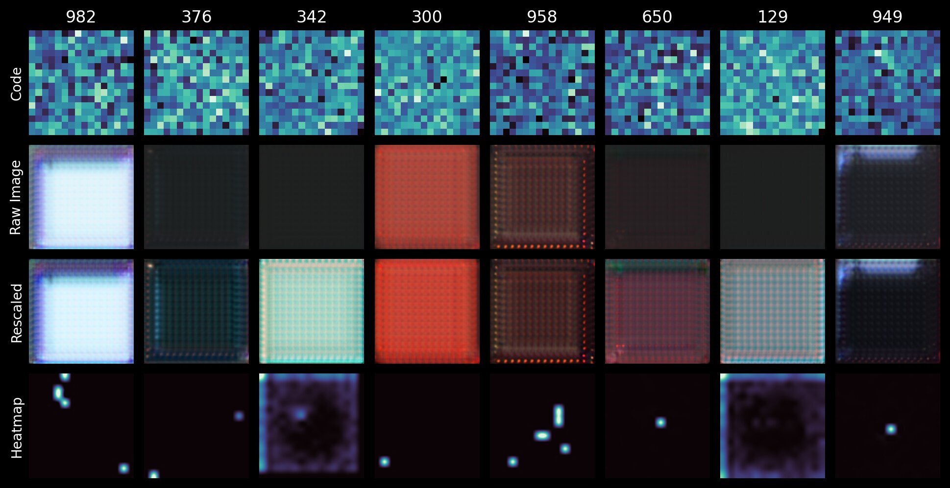
We can immediately see that some codes are highly localised; appearing only in specific regions of the latent tensor \( z \). By rescaling the images we can see that the codes that appear to produce blank space actually produce simple patterns. For indices 342 and 129, the spatial heatmap shows that they are more likely to be found on the edges of the latent map (it’s almost an inverse of a typical galaxy image). This strongly suggest that these codes (and these patterns) correspond to background space.
Conversely, the highly localised features and deliberate edge-like patterns of e.g. indices 982 and 949 correspond to the high-frequency structural components. Since 949 only ever appears in the center, it likely corresponds to a galaxy feature, while 982 likely corresponds to a star given it appears at the edge of the latent map. Remember that the spatial structure of the latent tensors \( z \) is the same as the input images \( x \); it’s merely downsampled by the encoder and quantized by the vector quantizer. This also means that any attempt to sample new z_quantized tensors must account for this topography; more on that later.
It should be clear now why changing the codebook size has the biggest effect on the fidelity of the reconstructed images. Each codebook vector corresponds to a feature (in much the same way as feature maps in a convolutional layer); the more codes, the more features you can encode. This links back to the idea of Voronoi tessellations: with more cells, you can better capture the underlying data distribution, while a coarser partition leads to these features averaging out (hence blurrier reconstructions). As with most things in ML, there’s diminishing returns, and a codebook that’s too large can fail to converge properly.
Wait, what about labels?
The Galaxy10 dataset does come with labels indicating the morphological classes, but we’ve barely mentioned them. Our VQ-VAE does not utilise them; it’s purely unconditional. This is all by design, since the role of the VQ-VAE is to strictly train an efficient codebook to capture the latent distribution of the inputs independent of any class conditioning. The class conditioning will come later in a second model that we will use to generate new images.
This doesn’t mean that the VQ-VAE is blind to labels; if anything it’s able to account for different class labels simply by virtue of unsupervised learning. Let’s perform dimensionality reduction via t-SNE on the sequences of codebook vectors and visualise the resulting embedding.
z_quantized_tsne = TSNE(n_components=2, perplexity=50, metric="cosine").fit_transform(
    z_quantized_list.reshape(z_quantized_list.shape[0], -1)
)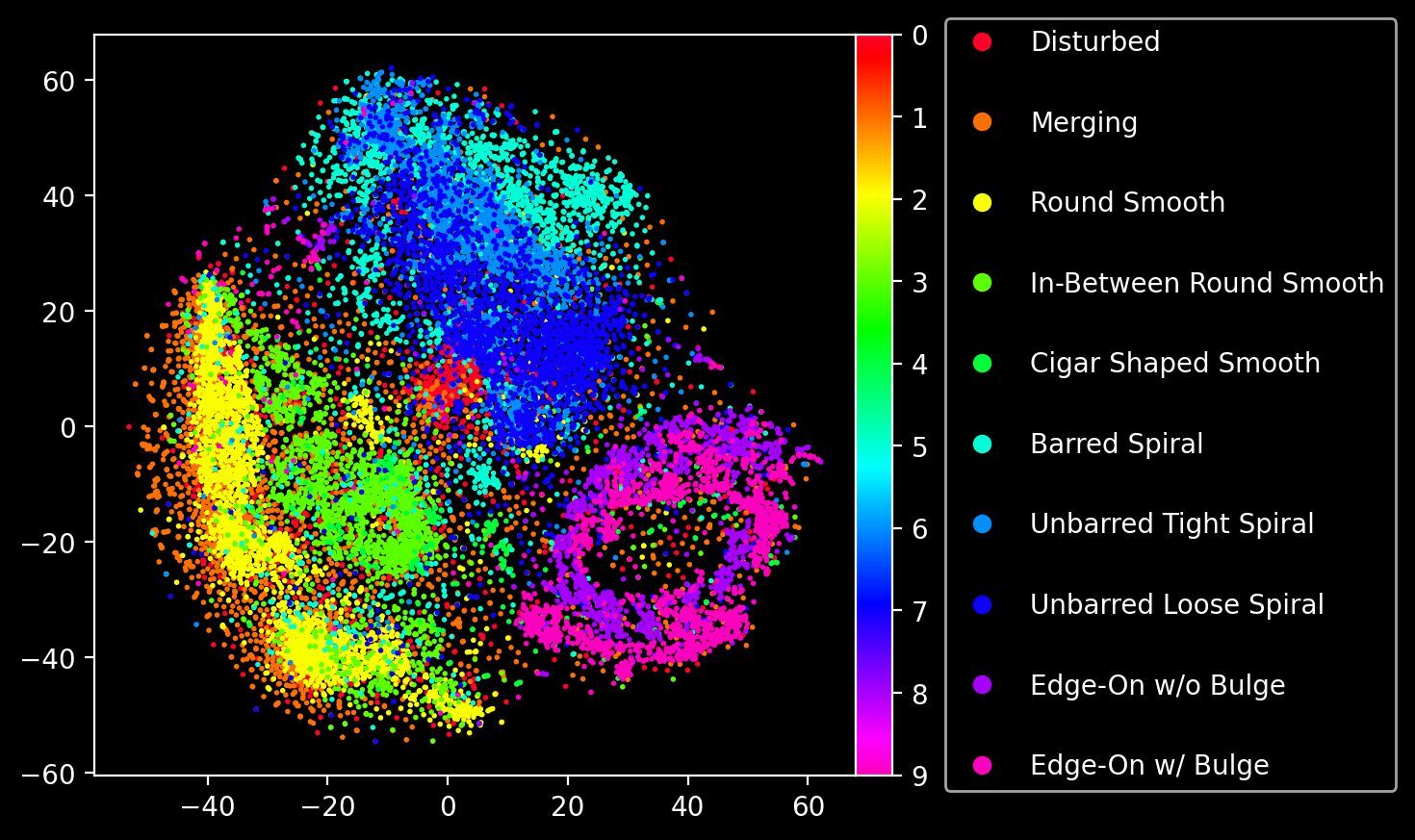
Like in our previous post on VAEs, we have arrived at a makeshift “morphological atlas” of sorts, showing how the model has learned (unsupervised) a latent representation that can separate different morphological categories.
The Need for a Prior
For regular autoencoders, creating new data is as simple as picking a random seed and running with it. For VAEs, just sample from the parameters of the latent distribution. For VQ-VAes, just pick random codebook indices, right?
Unfortunately this won’t work for VQ-VAEs. See for yourself:

Our input data is highly structured, and the VQ-VAE codebook is trained to represent this underlying data distribution. The sequences of codebook indices reflect this inherent, learned latent structure. Train a new VQ-VAE on the same dataset and you’ll get different sequences of indices. Furthermore, as we saw with the spatial heatmaps, the sequences of indices must reflect the topography of the original images. If you want to train a VQ-VAE to generate new data, then you also need a second model to generate realistic sequences of codebook indices that respect the learned structure.
One approach is to use PixelCNN, an autoregressive model that combines specialised masked convolutional layers to predict the next pixel in an image. This seems to be a perfect fit for our VQ-VAE as our codebook indices sequences are naturally structured as a 2D grid, but there are drawbacks. PixelCNN suffers from the same problems CNNs do: the limited receptive field. While you could use larger kernels or downsample to a smaller latent space, this severely impacts computational cost and model capacity respectively.
A better alternative is to use an autoregressive transformer-based prior for next-token prediction with the sequences of codebook indices directly. The mighty attention mechanism allows us to capture how each codebook index relates to all preceeding indices in the sequence rather than being confined to nearby pixels in the sliding window approach of PixelCNN.
A Conditional Transformer
Since we need a dedicated model to generate sequences, we can now finally get around to adding labels. There are several ways to incorporate labels into a transformer model, such as simply including a class token or adding a learnable class embedding to the sequence of tokens.
One of the more flexible methods is using class dropout, a technique where we train the model on both conditional and unconditional inputs (the latter of which is represented by a special null class). During inference, we can effectively employ classifier-free guidance (CFG). Here we run the model twice to obtain unconditional logits and conditional logits. The final, combined logits are simply logits = logits_uncond + cfg_scale * (logits_cond - logits_uncond) where cfg_scale is a strength parameter. You’re probably familiar with CFG from Stable Diffusion where it plays a similar role.
To start, let’s setup our nn.Module with what we’ll need:
class VQVAETransformerConditionalPrior(nn.Module):
    def __init__(
        self,
        num_tokens: int,
        embedding_dim: int,
        nhead: int,
        num_layers: int,
        latent_height: int,
        latent_width: int,
        num_classes: int,
        class_dropout_prob: float = 0.1,
    ):
        super().__init__()
        self.seq_len = latent_height * latent_width
        self.latent_height = latent_height
        self.latent_width = latent_width
        self.num_classes = num_classes
        self.class_dropout_prob = class_dropout_prob
Here num_tokens is the size of the codebook (number of codebook indices), which is essentially the vocabulary size for the transformer, while embedding_dim is the internal hidden dimensionality of the transformer (this is independent of the embedding dim used for the VQ-VAE codebook vectors). Since our sequence of tokens is a 1D array, it’s total length is equal to the dimensions of the latent grid of the VQ-VAE. We then store other parameters we expect to re-use. The class_dropout_prob is used to control the rate at which we randomly ignore input class labels. This ensures the model is trained with conditional and unconditional inputs.
Now let’s construct our key embeddings and learnable parameters:
self.token_emb = nn.Embedding(num_tokens, embedding_dim)
max_len = self.seq_len + 2
self.pos_emb = nn.Embedding(max_len, embedding_dim)
self.sos_token = nn.Parameter(torch.randn(1, 1, embedding_dim))
self.class_emb = nn.Embedding(num_classes, embedding_dim)
self.null_class_emb = nn.Parameter(torch.randn(1, 1, embedding_dim))
The token_emb is the main layer that maps each codebook index into vectors in the transformer’s own latent space of size embedding_dim.
Because our sequences of codebook indices have been flattened, we need to incorporate a positional embedding so that the transformer can account for the spatial context of each token. Notice that the sequence length for the positional embedding is max_len = self.seq_len + 2. This is because our sequence will have two additional prepended tokens:
[class_token] + [sos_token] + [token_0] + [token_1] + …
The SOS token is used to predict the first token in our actual ground truth sequence; the class token is hence used to condition the SOS token based on the current class label. We represent sos_token directly as a learnable parameter, whereas to encode our class information we use a nn.Embedding layer mapping the number of class labels to latent vectors. Because we’re doing CFG, we also need a special embedding to represent a “null” class in order to train for unconditional generation; this can just be a learnable parameter.
The transformer itself is as follows. Notice how we’re using nn.TransformerEncoderLayer since self-attention is all we need.
encoder_layer = nn.TransformerEncoderLayer(
    d_model=embedding_dim,
    nhead=nhead,
    dim_feedforward=embedding_dim * 4,
    dropout=0.1,
    batch_first=True,
    norm_first=True,
    activation="gelu",
)
self.transformer = nn.TransformerEncoder(
    encoder_layer,
    num_layers=num_layers,
)
This uses the usual dim_feedforward expansion factor of four and explicitly sets batch_first=True to keep tracking the shape easier. As always, nhead must divide embedding_dim evenly. We also use the GeLU activation function instead of ReLU. We need a few more layers to transform the output of the TransformerEncoder and complete our VQVAETransformerConditionalPrior.
self.to_logits = nn.LayerNorm(embedding_dim)  # to be applied before self.head
self.head = nn.Linear(embedding_dim, num_tokens, bias=False)
self.head.weight = self.token_emb.weight  # weight tying
Our output layer, head, is a simple linear layer mapping latent vectors to logits over the entire range of codebook indices. We also define an extra layer normalisation to be applied to the transformer output before passing through the head (this is why we set norm_first=True for the encoder_layer). Here we use a trick called weight tying, which essentially ensures that our token embedding and output layer share the same weights (and hence the same latent space). This not only reduces the total weight count, but also typically improves model generalisation.
Last but certainly not least, since we’re training the model to predict the next token, we need a causal mask to ensure that tokens can only ever attend to past tokens, never future tokens:
self.register_buffer(
    "causal_mask", nn.Transformer.generate_square_subsequent_mask(max_len)
)
The Forward Pass
Since our model is autoregressive and to be used for next-token prediction, we need to slice the input indices to remove the last token.
def forward(self, x: torch.Tensor, y: torch.Tensor | None) -> torch.Tensor:
    x_input = x[:, :-1]  # (B, T-1)
    x_emb = self.token_emb(x_input)
    sos_emb = self.sos_token.expand(B, 1, -1)
Our forward pass accepts two tensors; x is our (flattened) sequence of indices of shape (B, T) and y is our tensor of class labels. Our input thus has the shape (B, T-1) where T is the number of tokens in the sequence of indices. We pass this through the token_emb embedding, and also setup our start-of-sequence embedding.
Now we need to implement CFG dropout:
    # Determine which class labels to use as per CFG dropout
    if self.training and self.class_dropout_prob > 0:
        keep_mask = torch.bernoulli(
            torch.full((B,), 1 - self.class_dropout_prob, device=device)
        ).bool()
    else:
        keep_mask = torch.ones((B,), dtype=torch.bool, device=device)

    # Default to null classes and populate only the actual class labels to keep
    class_emb = self.null_class_emb.expand(B, 1, -1).clone()
    if y is not None and keep_mask.any():
        valid_y = y[keep_mask].long()
        class_emb[keep_mask] = self.class_emb(valid_y).unsqueeze(1)

    # Final sequence
    input_seq = torch.cat([class_emb, sos_emb, x_emb], dim=1)
During training, to ensure the model learns both conditional and unconditional inputs, we decide to randomly discard real class labels with some small probability self.class_dropout_prob (which we previously set to 0.1). This is done for each input in a given batch. We can implement this by constructing a binary mask keep_mask which determines which labels to keep and which to mask out. We initially populate the class_emb batch with the null class embedding, then insert the relevant class embeddings only for the valid classes based on the keep mask (notice if no labels are provided. The final input sequence is indeed a concatenation of the final class embedding, followed by the SOS embedding, and then the embedding of the indices tokens themselves (minus the last index token, of course).
Because our tokens have 2D structure, we need to apply our positional embedding. We do this by passing the sequences indices 0, 1, 2, … into the pos_emb embedding layer. (Alternatively we could also use a 2D version of the usual sinusoidal positional encoding).
    seq_len = input_seq.shape[1]
    pos = torch.arange(seq_len, device=device).unsqueeze(0)
    input_seq = input_seq + self.pos_emb(pos)
Our input_seq is ready to pass through the transformer:
    out = self.transformer(
        input_seq,
        mask=self.causal_mask[:seq_len, :seq_len],
        is_causal=True,
    )
    out = self.to_logits(out)
    logits = self.head(out)  # shape = (B, seq_len, num_tokens)
    logits = logits[:, 1:, :]  # skip class token
self.head projects the output back into the original vocabulary size of the VQ-VAE indices, so the logits have the shape (B, seq_len, num_tokens). However it’s important to skip the class token as its only job is to predict the SOS token (which doesn’t exist in our ground truth). This now correctly aligns our logits for next-token prediction: sos_token predicts the first target x0, t0 predicts x1, t1 predicts x2 and so on, until the final logit t[n-1] predicts the last target x[n].
Our loss function is nn.CrossEntropyLoss(). Here’s an example training step, showing how we derive our transformer input sequences directly from the VQ-VAE (assuming our batch consists of images x and class labels y):
    x, y = batch
    with torch.no_grad():
        z = vqvae.encoder(x)
        b, c, h, w = z.shape
        z_flat = z.permute(0, 2, 3, 1).reshape(b, h * w, c)
        _, indices, _ = vqvae.vq(z_flat)

    logits = model(indices, y)
    loss = loss_fn(logits.reshape(-1, logits.size(-1)), indices.reshape(-1))
We pass the raw images through the encoder to get the latent vector z, then flatten the latent grid to a sequence of length h * w. We extract the indices from the vector quantizer then pass this through the conditional transformer model (remember to also pass the class labels!).
It’s important to make the that the VQ-VAE is frozen: any operation that touches the VQ-VAE should use torch.no_grad(). Remember to also set vqvae.eval(). Since nn.CrossEntropyLoss expects 1D targets, we can reshape both logits and indices to flatten the batch dimension, which is fine as it allows us to treat each input as an independent next-token prediction problem.
Generating New Images
Hopefully you’ve kept up this far, but we’re still not actually done. Having created our conditional transformer prior and trained it for next-token prediction, we next need to create a function to generate new images. As this function is purely for inference, we decorate it with @torch.no_grad().
@torch.no_grad()
def generate(
    model: nn.Module,
    vqvae: nn.Module,
    num_generations: int,
    class_labels: torch.Tensor | None = None,
    cfg_scale: float = 3.0,
    temperature: float = 1.0,
    top_k: int = 0,  # optional; 0 to disable
    top_p: float = 1.0,  # optional; 1.0 to disable
) -> tuple[torch.Tensor, torch.Tensor, torch.Tensor]:
    model.eval()
    vqvae.eval()
    total_seq_len = model.seq_len
    latent_h = model.latent_height
    latent_w = model.latent_width
Having trained the prior with CFG gives us the flexibility to generate new images conditionally (with the desired class_labels tensor) or unconditionally. We can introduce a cfg_scale parameter to control the strength of the conditioning. Another useful parameter is temperature, which is a scale factor applied to the logits prior to sampling to determine how random / deterministic the resulting sequence is, along with two common filtering parameters: top_k and top_p.
Unlike in training, where we were able to parallelise the next-token prediction since we had the full sequence, for autoregressive inference we need to construct the new sequence token-by-token.
    generated_indices = torch.zeros(
        (num_generations, 0), dtype=torch.long, device=device
    )
    for _ in tqdm(range(seq_len)):
        # add dummy token
        dummy_token = torch.zeros((num_generations, 1), dtype=torch.long, device=device)
        x_in = torch.cat((generated_indices, dummy_token), dim=1)

        # cfg
        if class_labels is not None and cfg_scale != 1.0:
            logits_cond = self.model(x_in, class_labels)[:, -1, :]
            logits_uncond = self.model(x_in, None)[:, -1, :]
            logits = logits_uncond + cfg_scale * (logits_cond - logits_uncond)
        # purely conditional
        elif class_labels is not None:
            logits = self.model(x_in, class_labels)[:, -1, :]
        # purely unconditional
        else:
            logits = self.model(x_in, None)[:, -1, :]

        # sample new codebook index and add to sequence
        logits = logits / temperature
        logits = top_k_filter(logits, top_k=top_k)
        logits = top_p_filter(logits, top_p=top_p)
        probs = F.softmax(logits, dim=-1)
        idx_next = torch.multinomial(probs, num_samples=1)
        generated_indices = torch.cat((generated_indices, idx_next), dim=1)
We start off with an empty sequence. At the start of the loop, we append a dummy token. Recall how our transformer forward pass removes the last token to correctly setup the next-token prediction. If we didn’t add a dummy token then the model would just re-predict the latest token instead of predicting the next one.
The transformer has three modes: CFG, purely conditional (avoids the unnecessary unconditional generation if cfg_scale is 1) and purely unconditional. For CFG, we run the model twice to obtain a conditional and unconditional output, then extrapolate the difference based on the cfg_scale factor.
To actually select the next index, we need to sample the output logits. Prior to sampling, we apply our temperature setting to modify the logits distribution. We also pass the logits through optional Top-K and Top-P (nucleus) filtering. Top-K filtering is used to restrict the pool available options to only the top K most likely options (setting everything else to 0). Top-P filtering is used to restrict the pool of options to only those whose cumulative probability mass is at least the given threshold (where the options are sorted from most to least likely). Top-K effectively masks the original distribution of logits, while Top-P is used to trim the long tail of rare outcomes. One filtering is complete, we obtain our probabilities and sample our index using torch.multinomial. We append this index to the list, and repeat the process for the next index.
With the full sequence now complete, we can finally generate the actual image.
    indices_grid = generated_indices.view(num_generations, latent_h, latent_w)
    quantized = F.embedding(indices_grid, vqvae.vq.codebook)  # (b, h, w, c)
    quantized = quantized.permute(0, 3, 1, 2).contiguous()  # (b, c, h, w)
    images = vqvae.decoder(quantized)
    return images, quantized, generated_indices
We obtain the quantized vectors by sampling its codebook with our generated indices (rearranged as a grid). Note I’ve used F.embedding here to show how to directly sample the codebook rather than using the shorthand get_codes_from_indices, which generalises better to custom vector quantizers (and also works with arbitrary shaped tensors). We then need to rearrange the quantized vectors so that they can be passed into the VQ-VAE decoder.
After all those marathon steps, we finally have our fancy new images.
Unconditional vs. Conditional
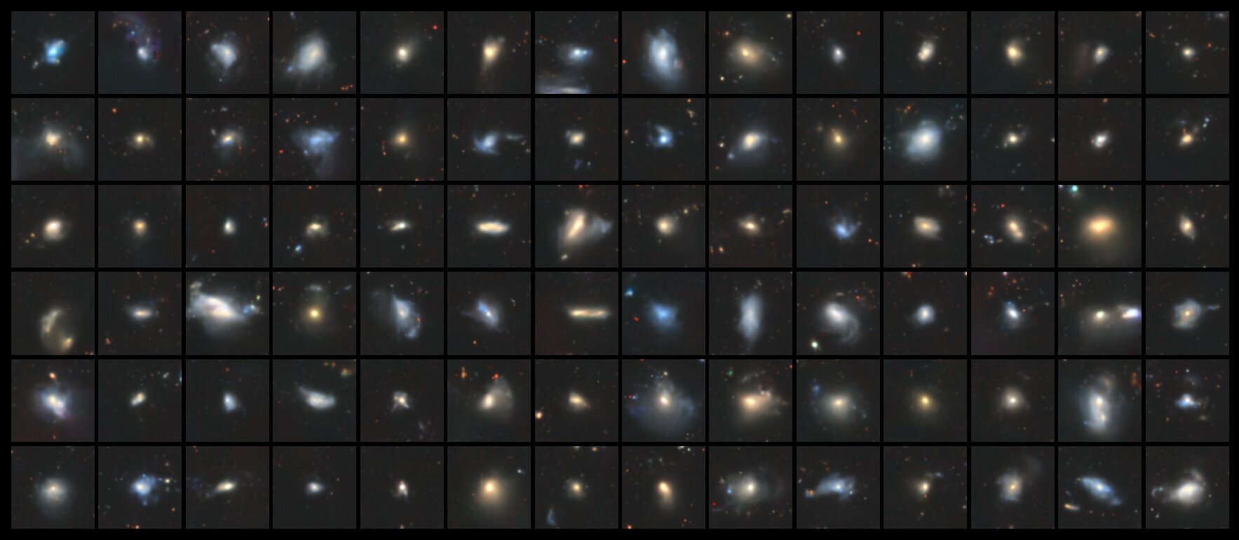
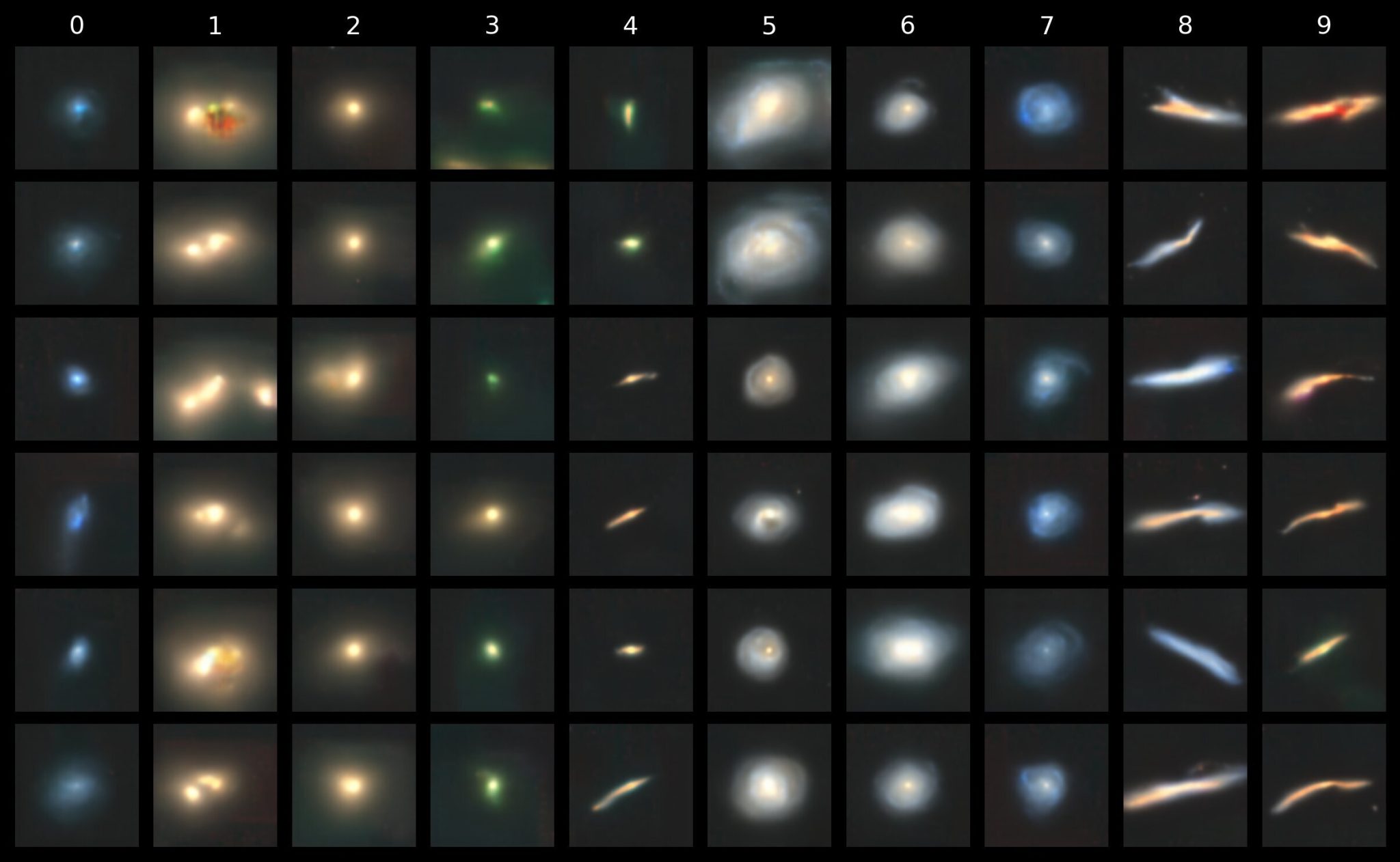
The example below shows unconditional images:
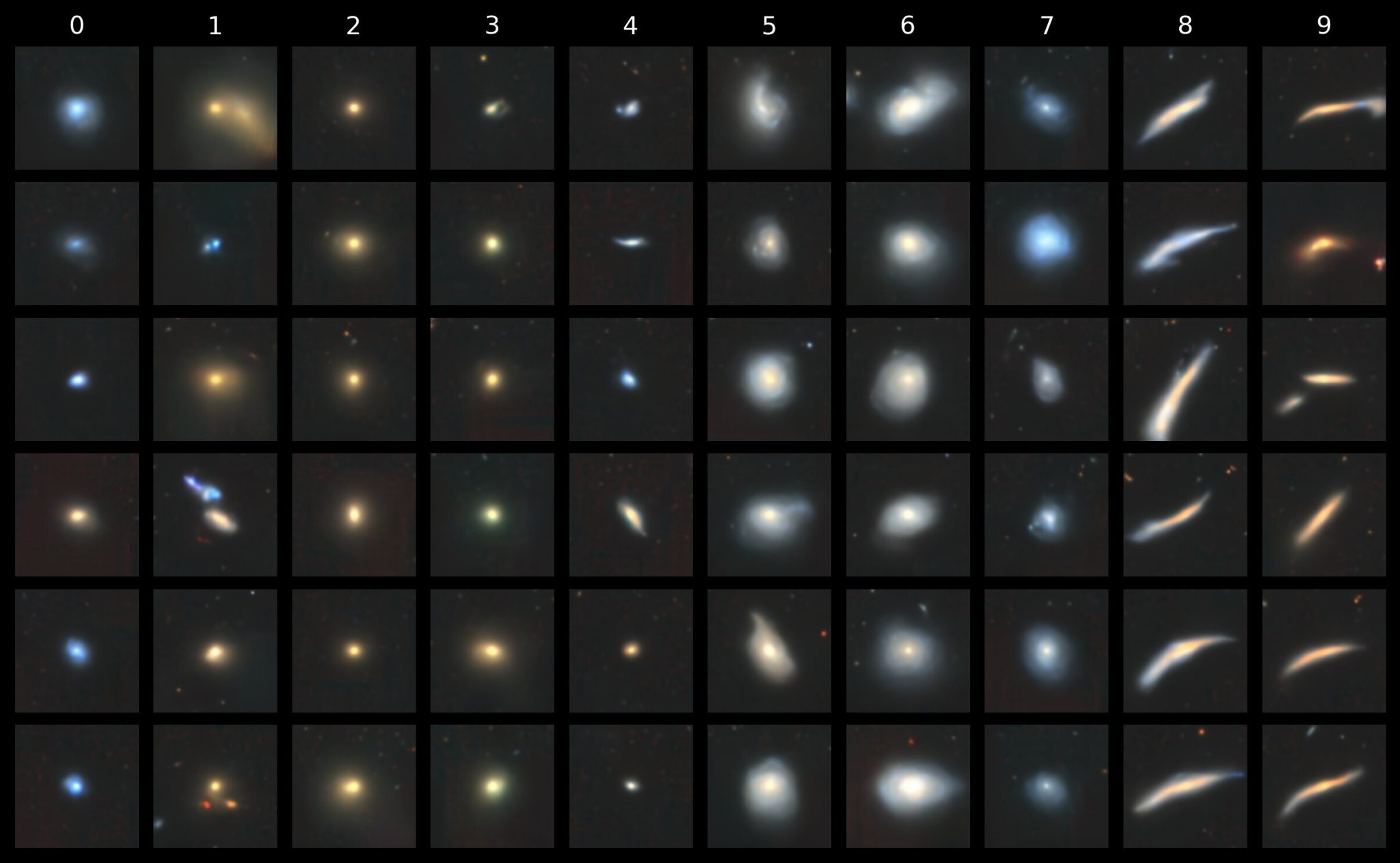
And now here’s one for conditional images (cfg_scale = 3). To save you scrolling back up to the start, the morphological classes from 0 to 9 are “disturbed”, “merging”, “round smooth”, “in-between round smooth”, “cigar shaped smooth”, “barred spiral”, “unbarred tight spiral”, “unbarred loose spiral”, “edge-on without bulge” and “edge-on with bulge”.

Cranking up the cfg_scale to 9 amplifies the class-specific characteristics, albeit at the cost of overall image cohesion:
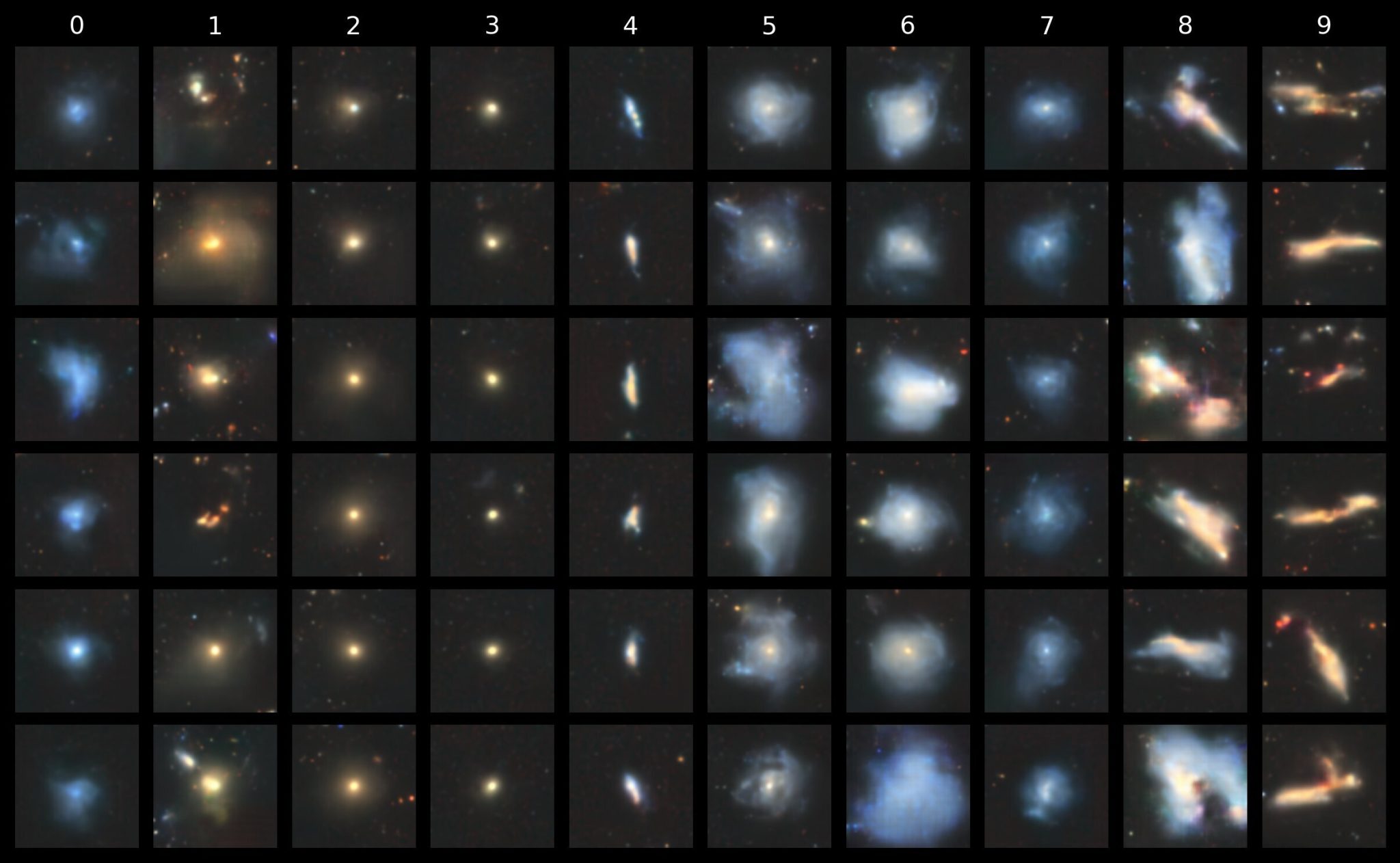
We can clearly see that this better captured the differences between tight and loose spirals and the characteristic shape in the “cigar shaped smooth” class.
And, for no reason other than the fact that we can, let’s see what happens with an absurd cfg_scale of 100. Notice how this severely restricts image diversity, with the outputs having instead converged to a relatively narrow set of features with severe artifacts. This is similar to what you typically see when mode collapse occurs in GANs.
Top K and Top P Filtering
Naturally, we might then inquire about which codebook indices are most important in distinguishing between the different morphological classes. Now that we have a conditional prior, that information is baked into the model itself. And it so conveniently happens that we included a top_k parameter in our generate function!
Let’s go with a top_k of 5. In other words, at each stage in the sequence generation loop, the choice for the next index is limited to only the top 5 highest logits (i.e. 5 most likely candidates relative to all others). What effect does this have on the images?
Quite a dramatic one! Because the indices are restricted to only the likeliest next-index choices, the resulting image emphasises the essential forms and features most relevant to the given class, without any superfluous features such as background stars or artifacts that were otherwise filtered out!
We get a similar result with using only Top-P filtering. The figure below shows what we get for top_p = 0.8 (i.e. restrict to the smallest set of tokens whose cumulative probability mass is at least 80% of the total when sorted from most to least likely).
Temperature and Diversity
There’s one more parameter we can tweak: the temperature. You’ve probably experimented with different temperature values when using LLMs in, say, Open WebUI or with paid APIs. Temperature is often defined as a parameter that controls the degree of randomness / determinism. Recall the way we apply it to scale the logits (prior to softmax) \[ \text{logits} = \frac{\text{logits}}{\text{temperature}} \] A low temperature amplifies the logits, leading to a sharper probability distribution after softmax that emphasis high-likelihood tokens. A high temperature instead reduces the logits, leading to a flatter probability distribution after softmax, meaning that there is greater chance of picking tokens that were originally less likely. Let’s see how this affects our galaxy images:
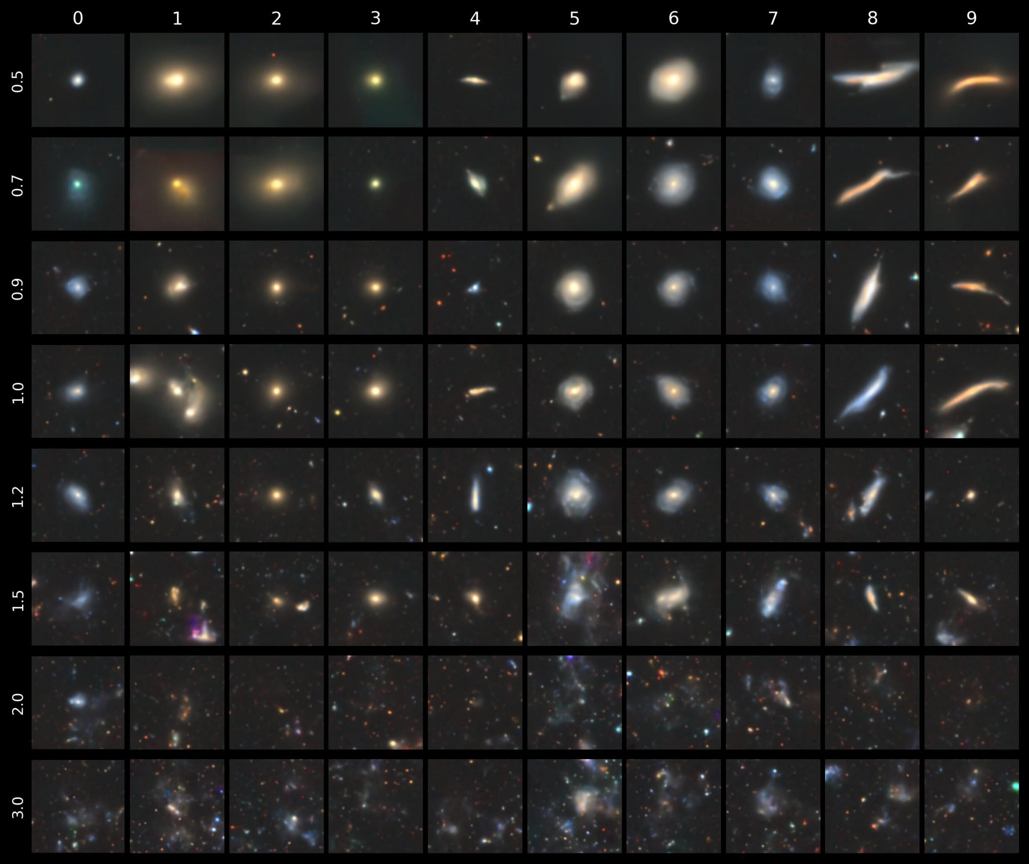
At low temperatures (around 0.5 and 0.7), the images resemble what we saw with the top-k and top-p filtering. Because we’ve amplified the probability distribution, the model selects from the (smaller) pool of high-probability logits, leading to more deterministic and repetitive outputs compared to the baseline. As we increase temperature from 1.0 to 1.2 and 1.5, we introduce more diverse features; background stars/galaxies are amplified and we see more purples and blues. However, at high temperatures beyond 2.0, the images become incoherent, instead resembling the images we saw when we gave the decoder a random sequence of codebook vectors. Indeed, as the temperature rises the probability distribution gets flatter (approaching the limit of a uniform distribution), and so the result becomes essentially random.
Latent Morphology
Now that we have a prior, we can effectively generate as many new images of galaxies as we want, for a given input class label. Yet do these images retain a semblance of structure? We saw in the purely unsupervised VQ-VAE that the latent space, when reduced to a 2D plane with t-SNE, was able to separate different morphological types fairly well. Has the conditional prior also managed to capture this latent representation? We can check this out by performing the same t-SNE dimensionality reduction procedure, but this time on the actual quantized codebook vectors that correspond to the sequences of codebook indices generated by our conditional transformer prior (this is why we also return quantized in our generate function!)

The separation is not as clean as what we saw with the main VQ-VAE, but there’s still a clear structure to the embedding.
You might think the outcome illustrated above is only possible because we used a conditional transformer prior trained with CFG. While class conditioning certainly makes visualising the different morphologies easier, the fact remains that the original sequences of indices (i.e. the training data for the prior) were generated from the VQ-VAE’s vector quantizer: an unsupervised model. The VQ-VAE has done the heavy lifting in obtaining a latent codebook representation of the Galaxy10 dataset. The conditional transformer prior then gives us the power to interpret (and eventually emulate) the latent space of the codebook by autoregressively training on the sequences of codebook indices. It is that step that can optionally benefit by conditioning on class labels. The base VQ-VAE is entirely unsupervised.
We chose to train the conditional prior on the original morphological class labels, but there is nothing to stop us from conditioning on other labels, perhaps even incorporating physical properties such as stellar mass, star formation rate and Sersic indices. Of course, since that would be a type of continuous conditioning, where the class labels are no longer discrete integers, you’d have to use a sinusoidal or Fourier-based embedding (like in neural radiance fields) rather than the linear/discrete nn.Embedding we used. If there is indeed a correlation, a conditional prior should reveal it (assuming a suitably powerful VQ-VAE).
Where lies galaxy morphology?
It’s a tad presumptuous to conclude this post with the question “where lies galaxy morphology?”, because this entire exercise in training a VQ-VAE on Galaxy10, even if it was 100% precise, could only ever tell us about the collective morphologies captured in Galaxy10. It will always be a challenge for any model, analytic or AI-based, to disentangle the true underlying galaxy morphology from selection biases or image characteristics (signal-to-noise, the method used to convert photometric bands to RGB, post-processing and compression artifacts, etc.).
For example, the James Webb Space Telescope has revealed distant galaxies have much richer morphological features than previously thought, yet that’s only because previous telescopes such as Hubble simply weren’t as powerful. So when it comes to exploring galaxy morphology with machine learning, a model can only ever be as good as the data it is trained on, and datasets can only consider so many galaxies.
Nevertheless, the fact that a VQ-VAE paired with a conditional transformer prior can reveal such strong morphological characteristics is encouraging. Even without the prior, we saw that the VQ-VAE was able to learn a latent codebook representation that successfully distinguished different morphological classes (as revealed by dimensionality reduction with t-SNE), all in an entirely unsupervised fashion.
VQ-VAEs, along with generative deep learning models in general, are thus viable tools for the classification and exploratory analysis of galaxy morphology, when trained on suitably large datasets of galaxy images. Several recent papers have explored this, including:
- Cheng, T. Y., et al., (2021): VQ-VAE + hierarchical clustering
- Robertson B. E., et al., (2023): Convolutional U-Net
- Semenov V., et al., (2024): Manifold learning (UMAP, t-SNE, etc)
- Tian C., et al., (2025): Transformer + CNN (GAN for preprocessing)
- Howie S., et al., (2025): VAE + PCA
- Ma C., et al., (2025): Stable Diffusion 1.5
And, of course, my papers have a bit to say about morphological classification too.
As larger datasets from next-generation surveys become publicly available, I bet that we’ll see even more studies apply generative AI techniques to reveal their latent morphological secrets.