When it comes to coding a convolutional neural network (CNN), how do you decide on a good architecture? You could, of course, adapt an existing, pre-trained model such as VGG16 or Inception v3, follow various online tutorials, or perhaps take inspiration from previous papers relevant to the kind of task you’re aiming to implement. In most cases, that’s enough to get by. But if you want to squeeze out the absolute best performance you can for the data you have on hand, you sometimes have to design from scratch.
Mining Order from Chaos
Deep learning is a field often described as more akin to alchemy rather than science, leaning on “best practices” and other heuristics based predominantly on experiments and real-world results as opposed to theory per se. That’s not to say that deep learning isn’t firmly rooted in linear algebra, optimisation and statistics – tangible, concrete mathematics – for it very well is.
Neural networks are vast information processors; each node in a layer of nodes applies a function to the weighted sum of all its preceding input nodes (plus a bias) and uses this to calculate an activation. This calculation is continued all the way to the output layer, whose activations are simply the “output”. This output is compared with the expected, desired output (a.k.a targets and/or labels) to calculate a loss, a way of quantifying the statistical “distance” between what we want the network to output compared to what it is actually outputting. This loss is backpropagated through all the layers in the network such that all the weights and biases are tweaked (via gradient descent) in order to minimise the loss in the next iteration. This process continues until the loss is suitably minimised (usually right before the model starts to overfit), at which point the network is regarded as “trained”. This is, of course, the oversimplified gist of how neural networks work (and I encourage you to read the excellent, free online book Neural Networks and Deep Learning for a thorough treatment of the fundamentals or, if you’re keen, Ian Goodfellow’s iconic Deep Learning textbook).
Modern deep learning methods employ incredibly elaborate architectures with everything from convolutions to residual connections to fancy Bayesian priors. Despite this veneer of sheer mathematical substance, neural networks are often regarded as “black boxes”; training data goes in, magic happens, and out comes the result. This tends to implicitly encourage a trial and error approach to conjuring CNN architectures. One is easily tempted to simply fiddle with values and/or add layers until one gets a better result. This so-called “gradient student descent” process is time consuming and inherently flawed; no different to stumbling around in the dark, or as Brian Moriarty would say, “mining order from chaos”. To free ourselves from this “labyrinth of delusion”, we can instead employ a smarter, automated approach to tweaking our CNNs. We can use hyperparameter tuning.
Getting Started: A Somewhat Modest CNN
In this post we’ll look at conducting hyperparameter tuning using both Optuna and KerasTuner in Python. A hyperparameter is any parameter that affects the architecture of the CNN (also referred to as the network topology), or the manner in which it is trained. In short, it’s anything that affects the performance of a model. Let’s kick things off with importing the packages we’ll need, starting first with Optuna, a general-purpose optimisation framework.
import numpy as np
import tensorflow as tf
from tensorflow import keras
from tensorflow.keras import layers
import optuna
Note as of April 2022, Optuna is not preinstalled by default on Google Colab instances. Simply run !pip install --user optuna (the ! denotes a bash command). Also ignore any error that says “module tensorflow.keras could not be accessed”; this is a known IDE typing issue with version 2.8 of TensorFlow and does not impact code functionality. If on Colab, be sure to use a GPU runtime!
We’ll be using the MNIST dataset of handwritten digits, which can be loaded and processed as follows:
(X_train, y_train), (X_test, y_test) = keras.datasets.mnist.load_data()
X_train = np.expand_dims(X_train, -1)/255.
X_test = np.expand_dims(X_test, -1)/255.
y_train = keras.utils.to_categorical(y_train)
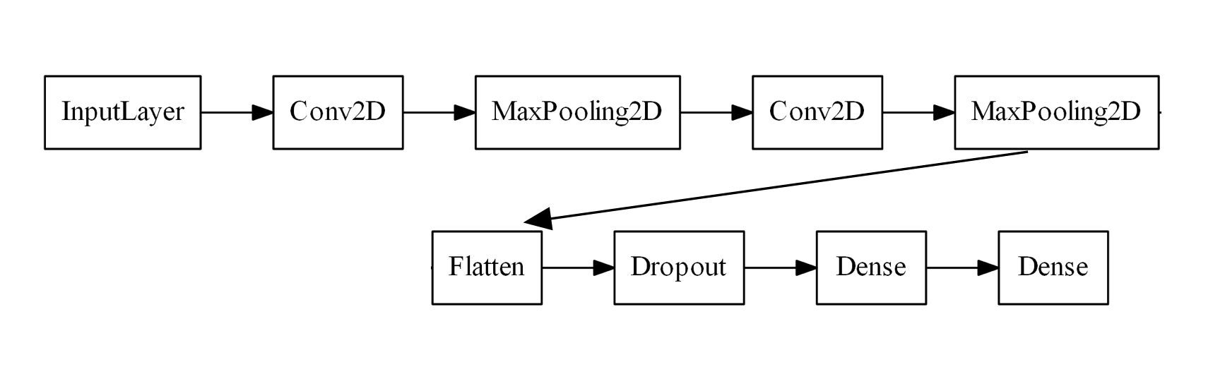
y_test = keras.utils.to_categorical(y_test)Let us now design a CNN. For this example, let’s use two alternating blocks of Conv2D layers and MaxPooling2D layers, followed by a Dropout layer, a Dense layer, and finally the output Dense layer.
As it stands, there are many values to potentially fiddle with. After all, what if we add another Dense layer or have three blocks of Conv2D layers? Let’s instead focus on more common hyperparameters, namely:
- The number of filters in each
Conv2Dlayer - The size of the convolutional kernel in each
Conv2Dlayer - The fraction of nodes to drop in the
Dropoutlayer - The number of nodes in the
Denselayer
Hyperparameters are not simply restricted to network topology; we can also change how the model is trained. In particular, we will alter the following:
- The learning rate of the Adam optimiser
- The batch size
This is by no means an exhaustive list of hyperparameters. For example, it may be worthwhile to consider the number of dense or convolutional layers as its own hyperparameter, utilise different activation functions, or even try AveragePooling2D layers instead of MaxPooling2D.
Optuna: Defining the Objective
Now that we’ve identified a set of hyperparameters, let us go ahead and define the objective function:
def objective(trial):
    keras.backend.clear_session()

    # build the model
    model = keras.Sequential([
        layers.Input(shape=(28,28,1)),
        layers.Conv2D(
            filters=trial.suggest_int('conv1_filters',32,64,step=8),
            kernel_size=trial.suggest_int('conv1_kernel',3,7,step=2),
            padding='same', activation='relu'
        ),
        layers.MaxPool2D(pool_size=(2,2)),
        layers.Conv2D(
            filters=trial.suggest_int('conv2_filters',64,128,step=16),
            kernel_size=trial.suggest_int('conv2_kernel',3,7,step=2),
            padding='same', activation='relu'
        ),
        layers.MaxPool2D(pool_size=(2,2)),
        layers.Flatten(),
        layers.Dropout(trial.suggest_float('dropout',0.1,0.5,step=0.1)),
        layers.Dense(trial.suggest_categorical('dense',[128,256,512]),'relu'),
        layers.Dense(10,'softmax')
    ])

    # compile it!
    model.compile(
        optimizer=keras.optimizers.Adam(learning_rate=trial.suggest_float('learning_rate',1e-4,1e-3,log=True)),
        loss=keras.losses.CategoricalCrossentropy(),
        metrics=['accuracy']
    )

    # now fit to the training data
    model.fit(
        X_train, y_train, batch_size=trial.suggest_categorical('batch_size',[64,128,256]),
        epochs=50, verbose=0,
        validation_data=(X_test, y_test),
        callbacks=[keras.callbacks.EarlyStopping(patience=3)]
    )

    loss, acc = model.evaluate(X_test, y_test, verbose=0)

    return acc
Here the variable trial is used to define hyperparameters via trial.suggest_float, trial.suggest_int and so on. The most important functions to remember are:
trial.suggest_int(name, low, high, step (optional), log (optional)).
For example,trial.suggest_int('test',2,10,step=2)will define a parameter namedtestand suggest values between 2 and 10 (inclusive) in steps of 2 (i.e. 2, 4, …, 10)trial.suggest_float. Same arguments astrial.suggest_int, but this time for floating point numbers. You should uselog=Trueif dealing with logarithmic values, e.g. when sampling between orders of magnitude.trial.suggest_categorical(name, [choice1, choice2, . . .]).
For example,trial.suggest_categorical('test',[10,30,60])will define a parameter namedtestand suggest a value of either 10, 30 or 60.
In the above function, we first construct our model, then compile it, and then fit it to the training data. We finally return the accuracy of the model after evaluating it on the test data. In general, the objective function should do everything you want the model to do, and then return the value(s) you want to tune. In the example above, we return the single variable acc (corresponding to the final accuracy of the CNN as evaluated on the test set), and so Optuna will treat this as single-objective optimisation. Optuna also supports multi-objective optimisation, in which case the objective function should return a tuple of values that you want to tune. Taken altogether, the possible suggested values for each parameter forms what is known as the parameter space, or search space.
Conducting the Search
First, let’s construct a new Optuna study using optuna.create_study
study = optuna.create_study(
    direction='maximize'
)
In our case, we want direction = 'maximize' as we are wanting to maximise the value returned by our objective function. We can now perform the hyperparameter tuning as follows using study.optimize:
study.optimize(
    objective,
    n_trials=50
)
Optuna will report on its progress, outputting the parameters used in the given trial, the value of the objective, as well as the best value seen across all trials thus far. Once the study is complete, simply run print(study.best_params) to see the optimal hyperparameters, and print(study.best_value) to see the best accuracy.
Visualisations
Optuna has several in-built plotting methods which offer some helpful insights into the nature of the parameter space. I’ll briefly cover the functions I found most useful:
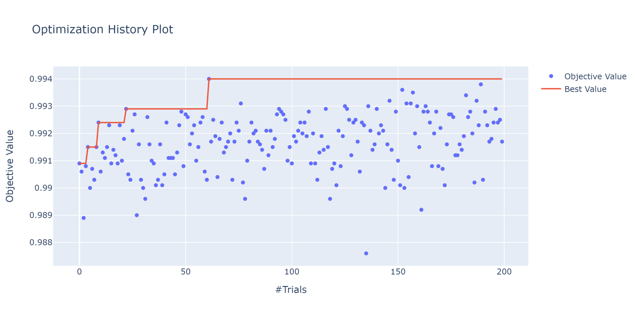
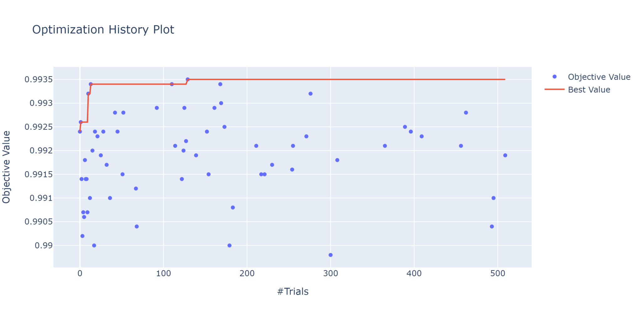
plot_objective_history
This is a quick way to view the performance of each trial, with the red line tracing the best value over time.
plot_parallel_coordinate
This is an excellent way to see which combinations of hyperparameters are better than others. It’s not as pretty as the hyperparameter sweep in Weights & Biases, but it gets the job done.
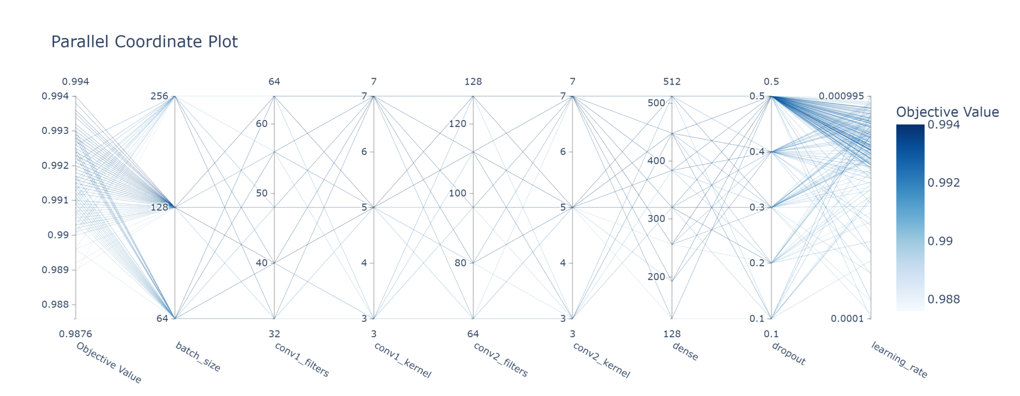
It’s also possible to visualise a subset of parameters, or even just one parameter, at a time.
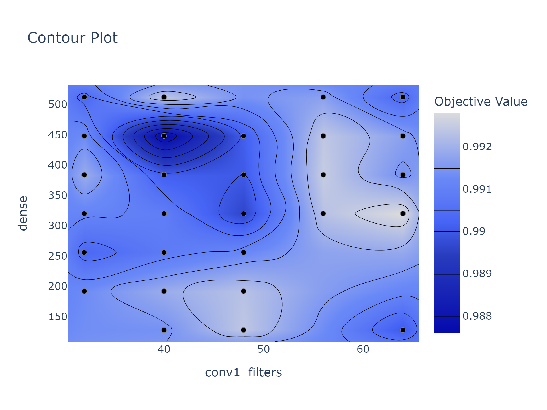
plot_contour
Allows you to directly contrast two parameters, and see which regions are optimal. In the below example, we can certainly rule out using 40 convolutional filters and 450 dense nodes, while 64 filters and 320 nodes is the best combination.
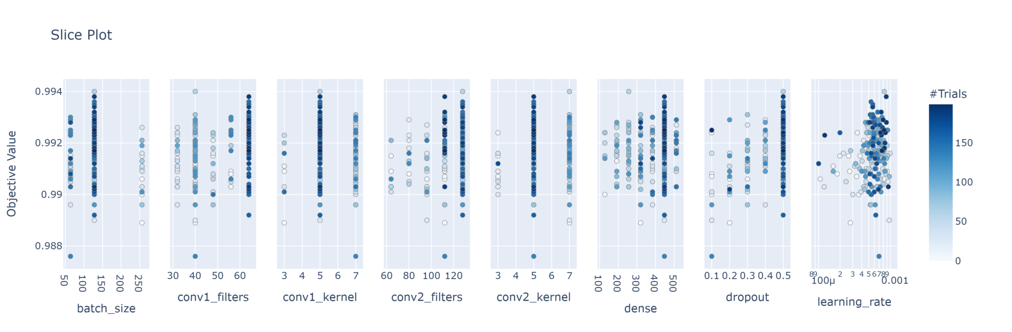
plot_slice
This plots the objective values of every trial for each parameter. Just like with the parallel coordinate plot, you can choose to instead plot only the parameters you want. Note the colouring is based on the trial number; darker colours indicate later trials.
plot_param_importances
This uses a random forest evaluator to determine which parameters are most important in influencing the objective.
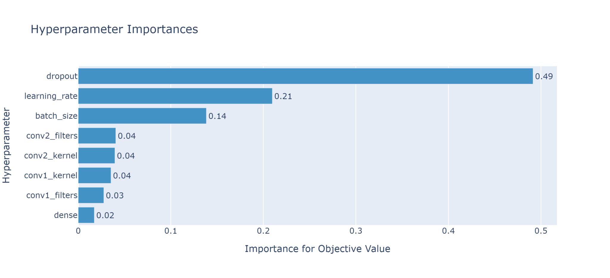
Based on the above plot, the dropout rate is the most influential parameter, while the number of nodes in the dense layer is least important (and could therefore potentially be removed from future fine tuning).
Pruning
One of Optuna’s greatest features, aside from the wonderful in-built visualisations, is its support for pruning. By pruning, we mean cutting short a trial when it is clear that it is underperforming. The term originates from classic AI, in particular the minimax algorithm with alpha-beta pruning, where (in, say, a game of chess) a search algorithm can safely ignore paths of a search tree that it knows are suboptimal (such as a move that any rational opponent would not possibly make). In the case of tuning CNNs, if the initial results of training are very poor, why bother wasting time training to completion? Instead, we can prune the search, and move on to the next selection of parameters.
To implement pruning, first add TFKerasPruningCallback to your list of callbacks:
model.fit(
    #...
    callbacks = [
        optuna.integration.TFKerasPruningCallback(trial,'val_accuracy'),
        tf.keras.callbacks.EarlyStopping(patience=3)
    ]
)
Then, when creating the study, add a pruner. In this example we use the standard MedianPruner, which prunes a trial if its best intermediate result is in the bottom 50% of previous intermediate results at a given step (in our case, at a given epoch).
Pruning allows for a much more thorough, yet narrow, exploration of a given parameter/search space. However, one should be careful not to prune too aggressively, for it’s possible that some trials could simply start off slow before eventually coming good later on (were they not pruned beforehand). This “horizon effect” is an inherent and unavoidable problem with pruning in general. Furthermore, pruning can potentially narrow the choice of parameters. Although you may be able to run many more trials in a given period of time, the parameter choices may be more constrained. This is, of course, by design; the default TPE sampler ranks pruned trials below completed trials, so there is necessarily less exploration of pruned parameter values. Thus, if you wish to thoroughly explore the entirety of the parameter space, it’s wise to use pruning sparingly.
Multi-Objective Optimisation
Optuna can attempt to optimise more than one objective at a time. In our example objective function, we returned the single value acc, and so all the hyperparameters were updated to try and maximise just this value. But neural networks aren’t simply all about accuracy. The loss is also important, as it quantifies how well the model is learning. In particular, it’s important to try and minimise the validation loss so as to avoid overfitting (which is what the early stopping callback is designed to do). In general, it’s the accuracy that matters most to real-world performance, but thanks to Optuna we can tune both the accuracy and the loss simultaneously through multi-objective optimisation.
This is as simple as modifying the objective function to return more than one variable:
def objective(trial):
    ...
    # rest of the code
    ...
    loss, acc = model.evaluate(X_test, y_test)
    return loss, acc
To define a multi-objective study, we use the directions argument.
study = optuna.create_study(
    directions = ['minimize', 'maximize']
)
Note that the directions (maximise or minimise) should be in the same order as the values returned in the objective function. In this example we are minimising the loss and maximising the accuracy.
There are a few caveats with multi-objective optimisation. You cannot prune trials, nor can you return any single best trial or best values. Instead, you end up with a list of best trials. This is by design as, in general, making one objective better often cannot be done without making the other worse. This concept is known as the Pareto efficiency, and the ideal solutions all lie on the Pareto front.
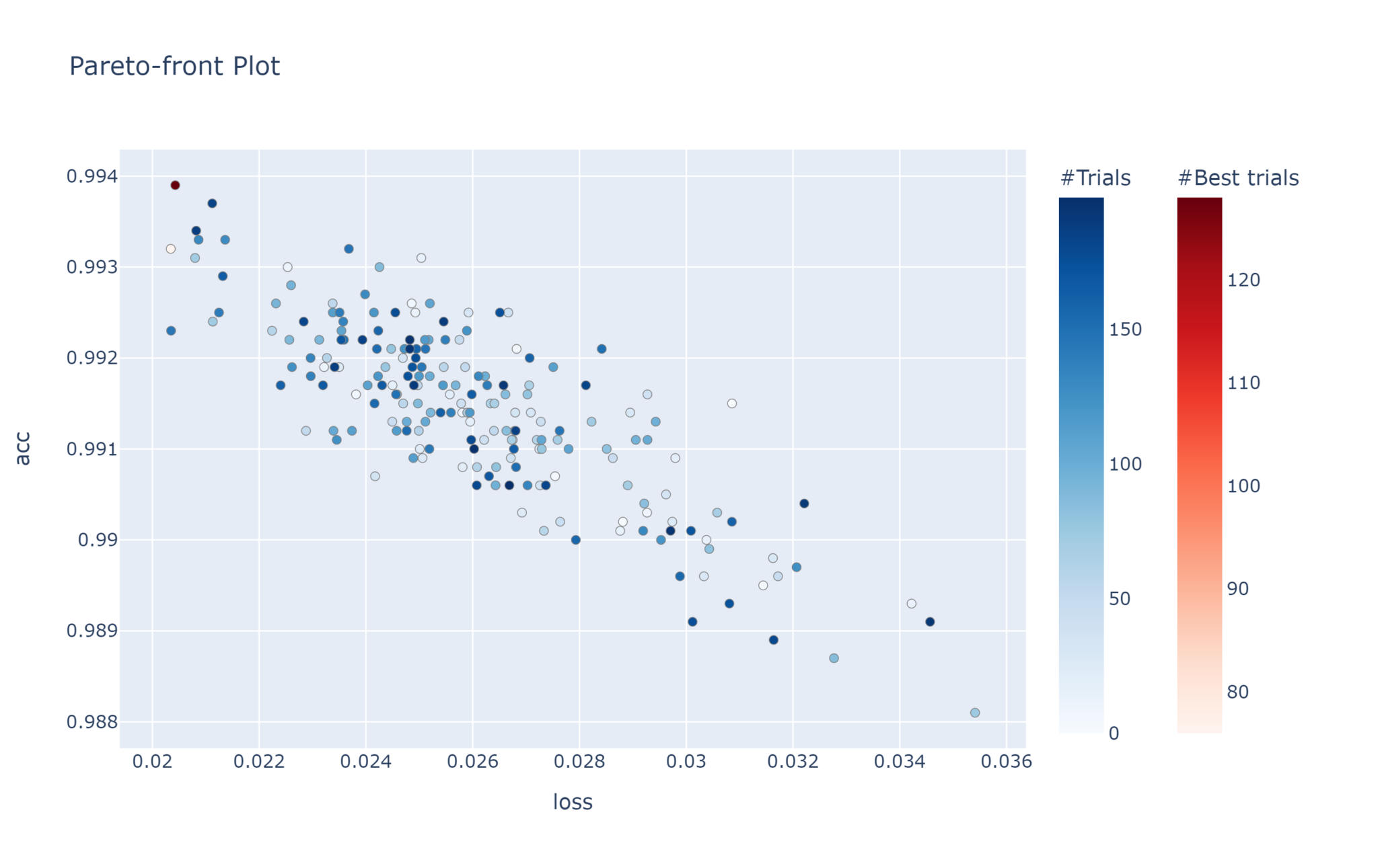
This plot allows us to see the relationship between the two objectives. Clearly, the lower the loss, the better the accuracy.
Samplers
One thing we have yet to mention is the method by which Optuna samples the search space. Optuna does this through dedicated Sampler objects. When defining a new study with optuna.create_study, and unless otherwise specified, the default sampler used is the Tree-structured Parzen Estimator (TPE) for single-objective optimisation, and the NSGA-II algorithm for multi-objective optimisation. TPE is a Bayesian optimisation approach which models probability distributions to calculate expected improvements, and henceforth selects parameter values that are most likely to improve the objective. NSGA-II is a genetic algorithm, in particular a type of elitist multi-objective evolutionary algorithm, which is noted for its speed and better convergence compared to similar alternatives. Optuna provides several other samplers, including:
GridSampler: Uses a “grid search” to methodically test all combinations of parameters.RandomSampler: Randomly samples parameter values from the search space.MOTPESampler: Multi-objective version of TPE.
KerasTuner: Building Keras Models
KerasTuner is a tool for hyperparameter tuning specifically designed for Keras. Simply install keras-tuner with pip, then add import keras_tuner as kt to your code.
KerasTuner’s workflow is different to Optuna’s. Whereas in Optuna you define an objective function and return some arbitrary value, in KerasTuner you are explicitly constructing, and returning, a Keras model. Let’s use the same CNN architecture and list of parameters as the above Optuna example, but this time written for KerasTuner:
def build_model(hp):

    model = keras.Sequential([
        layers.Input(shape=(28,28,1)),
        layers.Conv2D(
            filters=hp.Int('conv1_filters',32,64,step=8,default=64),
            kernel_size=hp.Int('conv1_kernel',3,7,step=2,default=5),
            padding='same', activation='relu'
        ),
        layers.MaxPool2D(pool_size=(2,2)),
        layers.Conv2D(
            filters=hp.Int('conv2_filters',64,128,step=16,default=128),
            kernel_size=hp.Int('conv2_kernel',3,7,step=2,default=5),
            padding='same', activation='relu'
        ),
        layers.MaxPool2D(pool_size=(2,2)),
        layers.Flatten(),
        layers.Dropout(hp.Float('dropout',0.1,0.5,step=0.1,default=0.5)),
        layers.Dense(hp.Int('dense',128,512,step=128,default=128),activation='relu'),
        layers.Dense(10,activation='softmax')
    ])

    model.compile(
        optimizer=keras.optimizers.Adam(learning_rate=hp.Float('learning_rate',1e-4,1e-3,sampling='log')),
        loss=keras.losses.CategoricalCrossentropy(),
        metrics=['accuracy']
    )

    return model
Note the similar yet slightly different syntax for selecting hyperparameters. There are also hp.Choice() and hp.Boolean() options, the former of which is analagous to Optuna’s trial.suggest_categorical().
Note that because this method returns a compiled Keras model, it is not possible to define training hyperparameters such as the batch size or number of epochs here. If you want to tune these, you have to instead define them in a custom kt.HyperModel class. Consider the below example:
class MyModel(kt.HyperModel):
    def build(self, hp):
        # same code as in the build_model(hp) method above

    def fit(self, hp, model, *args, **kwargs):
        return model.fit(
            *args,
            batch_size=hp.Choice('batch_size',[64,128,256]),
            **kwargs
        )

# Now use your custom class instead of build_model when creating the tuner
my_model = MyModel()
tuner = kt.Hyperband(
    my_model,
    # ...
)
For the rest of this post I’ll be sticking to the standard approach with build_model.
With the build_model(hp) method defined, let’s go ahead and initialise a tuner:
tuner = kt.Hyperband(
    build_model,
    objective='val_accuracy',
    max_epochs=20,
    hyperband_iterations=1,
    directory='testproject'
)
tuner.search_space_summary() # show summary of parameters
where search_space_summary() prints out a list of all the parameters and their range of values. Here we are using the Hyperband tuner, which uses the Hyperband bandit-based optimisation algorithm to find the optimal parameters. This is, of course, not the only tuner available, with the two notable alternatives being the RandomSearch tuner (for randomly choosing parameters) and the BayesianOptimization tuner (maximum likelihood estimation approach with Gaussians). Also note the directory argument; this is used to define a folder in which KerasTuner stores its checkpoints and logs (in this case, ./testproject). Note that this folder can get very big VERY quickly, especially for large models where 100+ gigabytes is par for the course, so this is something to keep in mind if running on a cloud instance and/or server with limited disk quotas (or if you’re super conservative about SSD writes). As of writing, there is no way to disable this, so if space is a concern then it’s best to keep runs small (or use Optuna).
To conduct the search, simply run the following:
tuner.search(
X_train, y_train,
validation_data=(X_test, y_test),
epochs = 20,
callbacks = [keras.callbacks.EarlyStopping(patience=3),keras.callbacks.TensorBoard("./tblogs")]
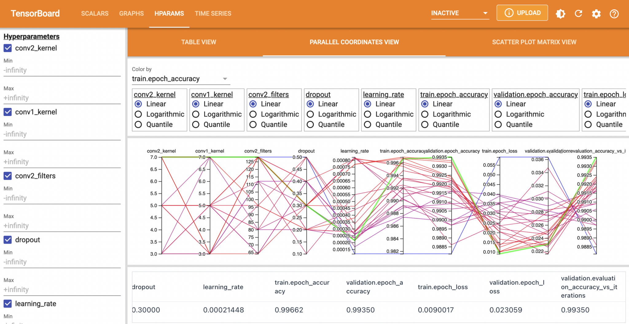
)Visualisation with TensorBoard
Although KerasTuner does not come with built-in visualisation methods like those in Optuna, we can still monitor the performance of the trials using TensorBoard. Simply ensure that there is a TensorBoard callback in your list of callbacks for tuner.search (or model.fit if subclassing), then open a terminal (ensure you’ve cd‘d to the current directory) and launch TensorBoard
tensorboard --logdir ./tblogsIf running on a local terminal, this should start a Python server with a link that you can paste into your browser. In Google Colab, you need to first load the TensorBoard notebook extension (note the % at the start of each command!)
%load_ext tensorboard
%tensorboard --logdir ./tblogs
Using TensorBoard with KerasTuner allows you to easily visualise hyperparameters, such as with its interactive parallel coordinates plot:
Conclusion
Both Optuna and KerasTuner are well and truly adept at optimising your CNN architectures. Optuna is a general purpose framework and uses an objective function that returns a value, while KerasTuner uses a model builder function that returns a Keras model. I personally prefer Optuna due to its simplicity and light overhead, storing trial results in RAM rather than writing tens of gigabytes, if not hundreds of gigabytes of checkpoints à la KerasTuner. That said, as with all things in life, you should go with whatever tool is best suited for your needs. Whether that be Optuna or KerasTuner is yours to decide. My hope is that this post has introduced the basics of how to get started with each.
References and Further Reading
- Optuna documentation
- KerasTuner documentation
- TensorFlow’s tutorial on KerasTuner
- Optuna examples (Github) for all sorts of platforms
- Neural Networks and Deep Learning, great online book
- Deep Learning by Ian Goodfellow et al.