The fifth of six posts covering content from SHPC4001 and SHPC4002
“On average, your friends are more popular than you.”
SHPC4001 Lecturer
In my undergraduate study at UWA, graph theory appeared very rarely and only in the context of algorithms, such as searching / traversal (BFS, DFS, A*, etc) and shortest paths (Dijkstra, BF). It also briefly reappeared in CITS2211 Discrete Structures in the context of topological sorts and partial orders. Network theory, which studies complex networks, can be considered as an umbrella discipline, of which graph theory is just one small part. A complex network is so named because they are often used to model real systems with non-trivial topological features (i.e a fancy way of saying that they are not your typical graph such as what you might use to illustrate an A* search). Complex networks are abundant in today’s information age, from social networks, communication networks and neural networks, to the Internet itself.
The SHPC4001 assignment involved constructing random networks (Erdős–Rényi model), small-world networks (Watts-Strogatz construction) and scale-free networks (Barabási-Albert model), then investigating (at least) one metric. This post will briefly cover all three network types, and explore several metrics including degree distributions, shortest paths, clustering and some common centrality measures. Also note that this post is restricted to simple, undirected graphs (no loops, edges can be traversed both ways). Without further ado, let’s delve into the world of complex networks.
Graph Fundamentals
Before exploring the three complex network models, let’s touch on how we describe networks (a.k.a graphs) mathematically. A network consists of a set of vertices \( V \) (also called nodes) and a set of edges \( E \) between these vertices. Mathematically, networks can be (and often are) represented using an adjacency matrix \( A \) defined such that \( A_{ij} = 1 \) if there exists an edge between vertex \( i \) and vertex \( j \), or 0 otherwise. This is all well and good, but in practice it is often more efficient to represent a graph using an adjacency list. An adjacency list is an array of size \( n \), where each index in the array contains a list of the neighbours of \( n \). If a node has no neighbours, then its entry is blank. Consider the following code showing how the two representations can be converted:
def matrix_to_adjlist(matrix):
    """Converts an adjacency matrix into an adjacency list"""
    size = len(matrix)
    assert size == len(matrix[0])
    #Here adj_list[i] will contain a list of neighbours to i
    adjlist = []
    for i in range(size):
        i_list = []
        for j in range(size):
            if matrix[i][j] != 0:
                i_list.append(j)
        adjlist.append(i_list)
    return adjlist

def adjlist_to_matrix(adjlist):
    """Converts an adjacency list into an adjacency matrix"""
    size = len(adjlist)
    matrix = np.zeros((size,size),dtype='int')
    for i in range(size):
        for j in adjlist[i]:
            matrix[i][j] = 1
    return matrix
The benefit of adjacency lists is that it is far easier to obtain the degree counts. We will say more about this in the metrics section, but the degree of a node is equal to its number of incident edges. In simple graphs with no loops, the degree is also equal to the number of neighbouring nodes / adjacent vertices (a loop – where a nodes is connected to itself, adds 2 to the degree count).
def degree_distribution_adjlist(adjlist):
    return [len(i) for i in adjlist]

def degree_distribution_matrix(matrix):
    return [sum(matrix[i][j] for i in range(len(matrix))) for j in range(len(matrix))]
See this StackOverflow post for a comparison of adjacency lists and adjacency matrices.
Erdős–Rényi
The Erdős–Rényi model is used to construct random graphs, i.e networks where the edges are randomly assigned between nodes. There are two equivalent models with which to construct a random graph: G(n,p) and G(n,M).
G(n,p)
Here we first initialise an empty matrix (of size n), then assign edges between nodes with a probability p. This last bit is important; it does not say that each node has a probability p of being connected to some other node, but rather it says that each unique edge (out of all possible edges) is assigned with a probability p. So \( G(10,0.1) \) would result in a graph with 10 nodes, such that every possible edge has a 10% chance of being assigned. The maximum number of edges in a graph with \( n \) nodes is \( n(n-1)/2 \).
G(n,M)
The G(n,M) model creates a graph with \( n \) nodes, randomly populated with \( M \) edges. So \( G(20,50) \) results in a graph with 20 nodes and 50 (random) edges. Note that \( M \) must be no greater than \( n(n-1)/2 \). An easy way to implement this is to loop M times, each time picking a random pair of unconnected nodes and assigning an edge between them.
In practice, the G(n,p) method is superior as it is significantly easier to scale, rather than having to keep adjusting the value of M whenever n is changed.
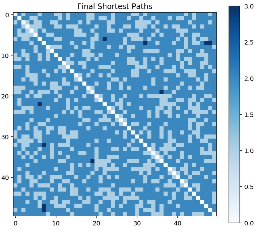
Another way we can visualise the randomness of the graph is with a matrix of shortest paths (where each entry \( i,j \) is the length of the shortest path from \( i \) to \( j \) ).
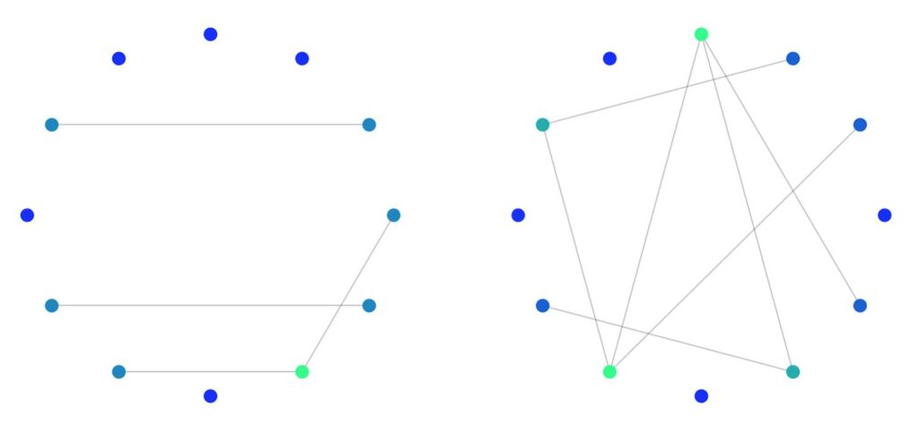
Giant Component
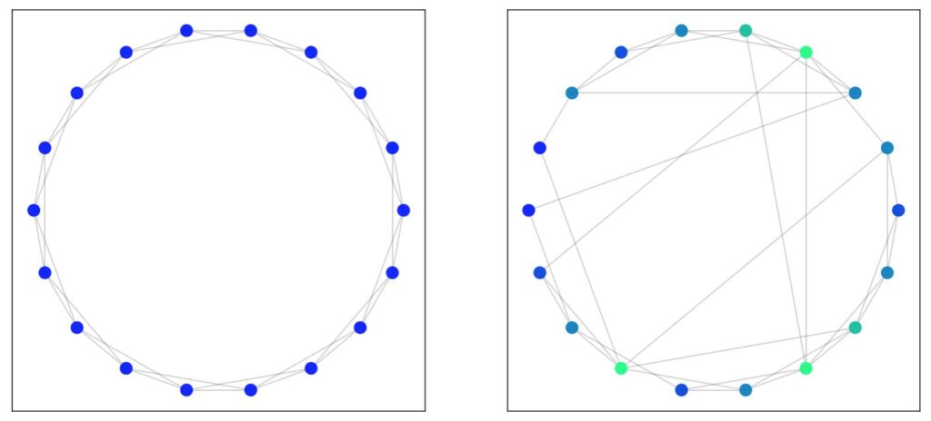
One of the distinguishing features of the Erdős–Rényi model is the presence of a giant component when the number of edges \( M \) exceeds \( (n-1)/2 \). This giant component can be thought of as the dominant internal component of the graph that connects the majority of nodes. So for a graph with 12 nodes, we expect a giant component to emerge with roughly 6 edges (this is where the G(n,M) construction comes in handy). Below is a plot of a random 12-node graph with 4 edges and 7 edges.
Watts-Strogatz
The Watts-Strogatz model is a means of constructing a small-world network; i.e a graph that is distinguished by high clustering but with a low diameter. Clustering can be thought of as related to the number of triangles in the network (relative to all possible triplets of edges), while the diameter of a graph is the maximum shortest path between any two nodes. In a small-world network, most nodes are connected to other nodes in their immediate surroundings, but any node can be reached in only a few number of steps. How does this work you might ask? It works by the use of shortcut edges (similar in principle to wormholes) that connect regions within the network that would otherwise have required many steps to reach.
In the Watts-Strogatz model of construction, we start with a ring lattice of \( n \) nodes such that each node is connected to \( K \) total neighbours (i.e \( K/2 \) neighbours on each side). The next step is to iterate over all the edges, and randomly reassign them with some probability \( p \) (also called the rewire probability). The end result is a partially broken-up ring with “shortcut edges” or wormholes that jump to the other side.
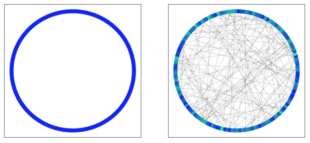
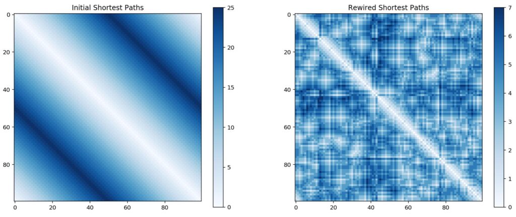
The idea here is that nodes that would otherwise only have been reached by traversing around the ring can instead be reached by travelling along a shortcut edge to reach the other side of the ring (like a wormhole). We see this most dramatically by examining the matrix of shortest paths.
Six Degrees of Separation
In the example below, we have a lattice of 100 nodes with each node connected to 2 neighbours on either side. As expected, given the lattice structure, nodes close together are easy to reach, while nodes located on opposite sides of the ring take up to 25 steps to reach. By introducing shortcut edges, we can jump across large swathes of the lattice, reducing the overall diameter of the graph (in this case from 25 to 7). This is the essence of the idea of six degrees of separation (although in this particular case it’s 7); that nodes that would otherwise appear to be extremely distant are actually easily reachable. While your social network may primarily consist of people in Perth, Australia, one of your friends might happen to know someone from New York.
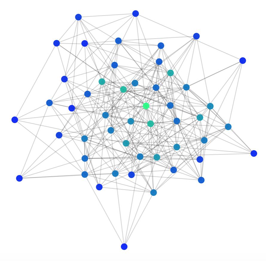
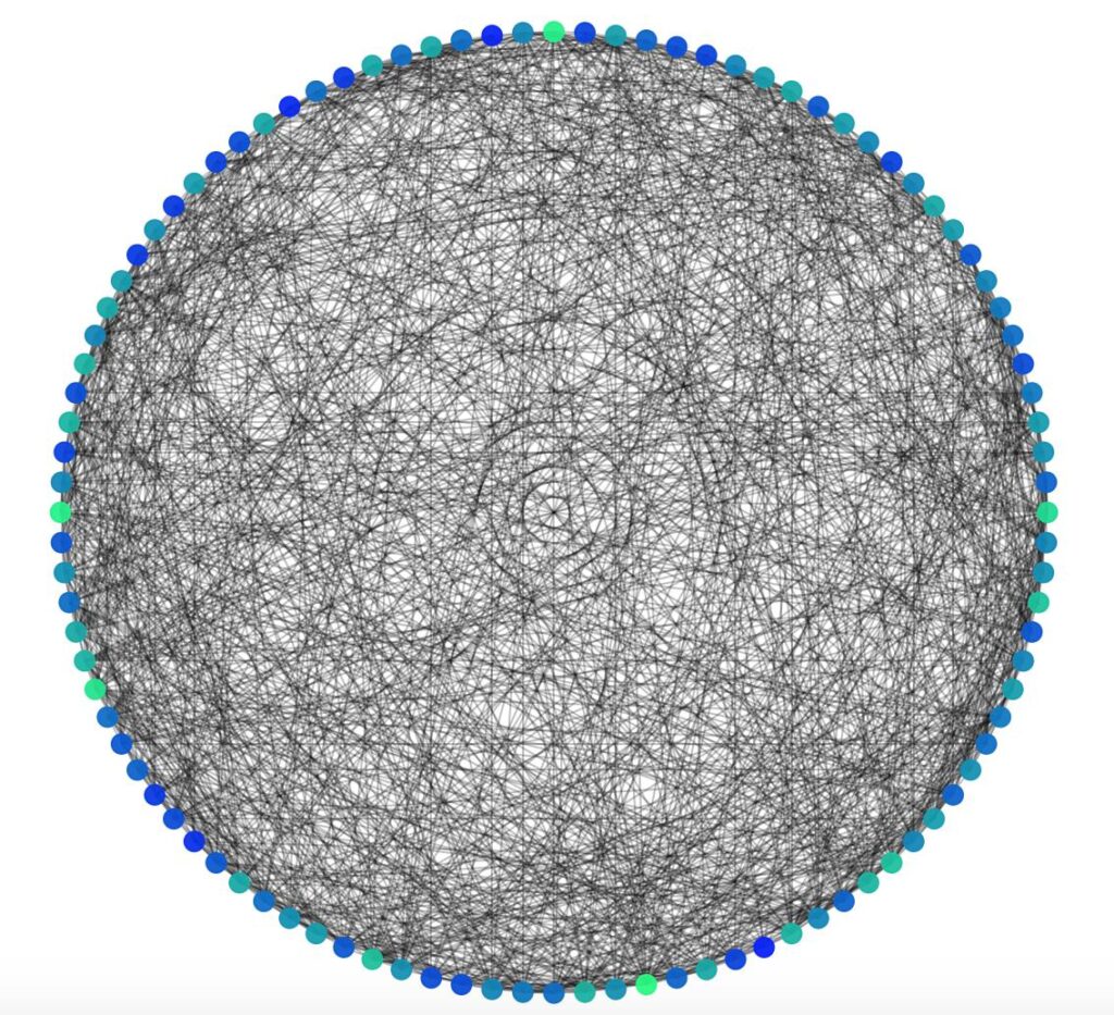
Barabási-Albert
The Barabási-Albert model is a method of creating a scale-free network by means of preferential attachment. Scale-free networks are characterised by a degree distribution that follows a power law (i.e when some quantity \( y \) is proportional to \(x^p \) for some power \( p \) ) . An example is a network where a few nodes have a high degree (and account for most of the edges) but most other nodes have a low degree (like, you know, wealth distribution). One way of creating such a method is the preferential attachment model of Barabási-Albert. Like the Watts-Strogatz model, it starts off with a pre-constructed graph. In this case, we start with a random Erdős–Rényi graph. The next step is to add new nodes to the graph, one at a time, such each new node is to be connected to \( m < n \) existing nodes. This generative step can be repeated any number of times. The trick here is that instead of merely populating these new edges randomly, we instead use a probability that is proportional to the degree of the node. So if there are 3 nodes, one with degree 2 and the others with degree 1, the node with degree 2 is more likely to receive the new edge. Thus new nodes are more likely to attach themselves to existing nodes with higher degree counts. The probability that a new node will attach to an existing node \( i \) is given by \[ p_i = \frac{k_i}{\sum_j k_j} \] where \( k \) is the degree of the node. Thus, for the 3 node example, the new has a 50% chance to attach itself to the existing node with degree 2, and a 25% chance to attach itself to the other two nodes with degree 1.
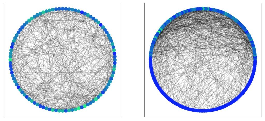
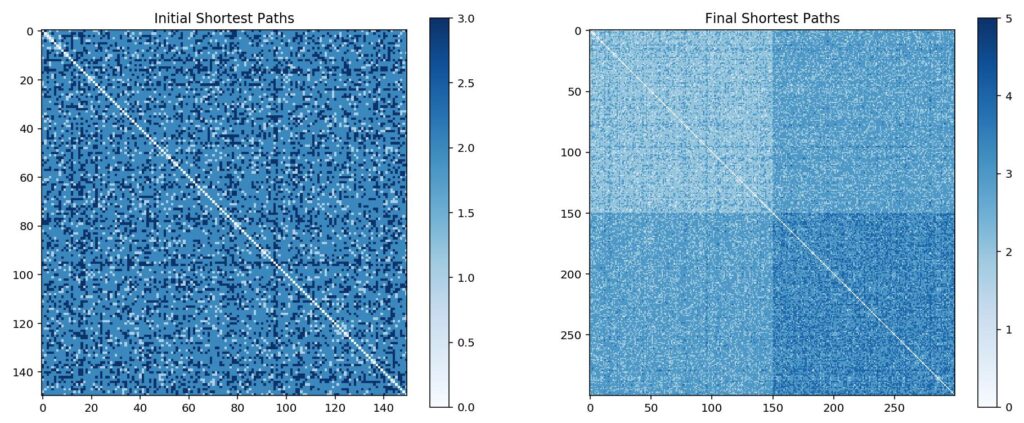
The best way to visualise this is with a large number of nodes. In the example above, we started with 150 nodes, then added an additional 150 using preferential attachment. The majority of new edges are with the original nodes, while almost all the newer nodes are left with relatively low degree counts. Similarly, a handful of nodes dominant with very high degree counts. It’s also useful to see how preferential attachment affects shortest paths:
Metrics
The key difference between complex networks and your everyday graph is that the former has non-trivial topological features. In the case of scale-free networks, the degree distribution is represented by a power law. Small-world networks are characterised by a high clustering coefficient, but a low diameter. Let’s now go over some key graph metrics (this list is by no means exhaustive).
Degrees and Density
In an undirected network, the degree of a node (usually the symbol \( k \) ) is simply the number of edges connected to it. We typically want to find the average degree of all nodes in a network; this is denoted as \( c \) in the literature: \[ c = \frac{1}{n} \sum_{i=1}^n k_i \quad k_i = \sum_{j=1}^n A_{ij} \] It follows that the mean degree is related to the total number of edges \( m \) via the following \[ c = \frac{2m}{n} \] This is particularly useful when calculating the density \( \rho \) of the network: \[ \rho = \frac{m}{\begin{pmatrix}n \\ 2\end{pmatrix}} = \frac{2m}{n(n-1)} \approx \frac{c}{n} \] The density can be thought of as the probability that any two nodes will be connected by an edge (a density of 1 implies that the network is fully-connected).
Also of interest is the degree distribution, often visualised as a histogram showing the frequencies of various degree counts. For random graphs, this distribution should be a normal distribution, while the scale-free graphs should show a skew typical of a power law. In the opening quote, I quoted my lecturer who said that your friends are more popular than you. This is one way of stating the friendship paradox, which is so called because the average degree of the neighbour to a node n is higher than the average degree of n itself. This is counter-intuitive (after all, shouldn’t all nodes have the same average degree?), but occurs because neighbours overlap when counting averages; a node with degree k will occur in k averages (as there are exactly k nodes connected to it). Thus high-degree nodes skew the average.
Shortest Paths and Diameters
The shortest path between two nodes is, well, the path that traverses the fewest edges (this is also colloquially referred to as the distance). A network’s diameter is the maximum length of all the shortest paths between all pairs of nodes. I found that the best way to visualise the shortest paths of networks as a whole was to compute a matrix such that each entry \( ij \) is equal to the length of the shortest path from \( i \) to \( j \). This can be done using a slightly tweaked Bellman-Ford algorithm:
def belman_ford(g, s):
    """g is a networkx graph"""
    distance = [0 for x in range(len(g.nodes))]
    for n in g.nodes():
        distance[n] = size
    distance[s] = 0

    for i in range(len(g)):
        for u in g.nodes():
            for v in g[u]:
                if distance[u] + 1 < distance[v]:
                    distance[v] = distance[u] + 1
    return distance
Note the code above uses the networkx package.
Connectivity
Of course it is not just the shortest paths that are of interest. Nodes can typically be reached by traversing multiple different paths. Some of these paths may traverse along the same edge, or pass through the same node. We call two paths edge-independent if they don’t travel along a common edge; and node-independent if they do not pass through a common node. The connectivity of a pair of nodes is equal to the number of independent paths between those nodes. This is also known as edge connectivity or node connectivity depending on which independent paths are the focus.
Centrality
There exist many centrality measures that all set out to answer the same question: which node is most important?
- Degree centrality is a simple measure that uses the degree of a node as a measure of its centrality. This turns out to be rather effective in the study of social networks (where the person with the most friends is usually the most important).
- Eigenvector centrality can be thought of as an extension to degree centrality that takes into account connections to nodes that are themselves more important (i.e if your friends are important then that makes you important). There are quite a few quirks and nuances that go beyond the scope of this post; suffice to say that you must use the “correct” eigenvector where the definition of “correct” is dependent on the problem you wish to solve.
- Katz centrality is similar to eigenvector centrality, although we introduce two constants \( \alpha \) and \( \beta \) such that the Katz centrality is calculated as: \[ x_i = \alpha \sum_j A_{ij}x_j + \beta \] If you think this equation looks like it’s suited to neural networks, you’re not wrong. One important variant of the Katz centrality is Google‘s PageRank, one of the algorithms it uses to rank web pages in its search engine.
- Closeness centrality aims to determine which node is closest to all others by analysing the mean distances (i.e the shortest paths), the idea being that the most influential node is the one with the fewest number of steps to all other nodes. There are two main ways to determine this mean distance: (1) using the simple average, or (2) using the harmonic mean.
- Betweenness centrality aims to determine which nodes lies on the most paths between all other nodes. Unlike the above centrality measures, the betweenness centrality does not take into account how many edges the node has (a node can have a low degree but high betweenness, such as a node that acts as a bridge between two larger regions).
Clustering, Cliques, Cores and Components
The clustering coefficient is defined as the fraction of all triplets that are closed (i.e the edges form a triangle). Thus a network with high clustering has many loops (often the case for social networks where your friends are typically friends with your friends-of-friends). A set of nodes such that each node is connected to every other is called a clique. A set of nodes such that each node is connected to (at least) \( k \) other nodes is called a k-core. Furthermore, we call a set of nodes such that each is reachable by a path through the other nodes a component (NB: components and cores are not the same thing!)
There are many other aspects of complex networks, from percolation and robustness, to reciprocity (in the case of directed graphs), and to modularities and communities, more than can be fit into a single blog post! For more on this wonderful topic, consider the textbook Networks by Mark Newman, or any other of the many complex networks textbooks out there.