The third of six posts covering content from SHPC4001 and SHPC4002
SHPC4001 is, first and foremost, the first core unit of the Computational Physics specialisation of UWA’s Master of Physics course (as well as a recommended unit for any pathway that requires some degree of programming). Naturally, quantum mechanics was to appear at some point. Over the course of two assignments, there were three problems that each involved solving the Schrödinger equation, firstly using the shooting method (for a 1D potential), secondly using the Numerov-Cooley method (also for a 1D potential), and finally using the direct matrix method (for a 2D potential). This post will briefly cover these three methods. As with the previous post on Numerical Methods, some familiarity with calculus is assumed, as well as an appreciation for quantum mechanics. Let’s briefly go over the basics before delving into the numerical methods.
TISE
Matter exhibits both particle and wave-like qualities, and this duality is one of the core foundations of quantum mechanics. Particles can be described by a wavefunction, usually denoted \( \psi(x) \), which is a (complex-valued) function satisfying the Schrödinger equation that encodes the probability of locating the particle within some region (there is much more to this, but that is beyond the scope of this post). It is a necessary requirement that \[ \int_{-\infty}^\infty | \psi(x) |^2 = 1 \] i.e the wavefunction is normalised (i.e the particle has to be somewhere). A common problem in quantum mechanics is to solve for the wavefunction in a given potential \( V \). For this post we will restrict ourselves to time-independent potentials \( V(x) \), and for now we will deal with 1-D potentials. Just as vibrations on a string or other mechanical system can cause standing waves, so too can we find stationary states for a quantum system. To solve for these, we use the Time-Independent Schrödinger Equation (abbreviated TISE) that, for a 1-D potential, is: \[ -\frac{\hbar^2}{2m} \psi^{\prime\prime}(x) + V(x)\psi(x) = E\psi(x) \] which is also commonly written as \[ \hat{H}\psi(x) = E\psi(x) \]
where \( \hat{H} \) is the Hamiltonian (operator). Those familiar with linear algebra will recognise that valid solutions \( \psi(x) \) are eigenstates (also known loosely as eigenfunctions) of the Hamiltonian with eigenvalue E. These eigenvalues correspond to the allowed quantum energies within the system, and the eigenstates form a basis for permissible wavefunctions through superposition (for more on this topic, consider an introductory quantum mechanics textbook such as Griffiths).
The Shooting Method
Let us consider a potential well, centred on the origin, such that as \( x \to \pm\infty \), \(V(x) \to \infty \) (i.e the potential becomes infinitely large the further away we go from the origin \( x = 0 \)). Thus our wavefunction \( \psi(x) \) must approach 0 the further away we go from the origin. Let’s consider, without loss of generality, some arbitrary interval \( [-a,a] \) where \( V(-a) \) and \( V(a) \) are sufficiently large for \( \psi(\pm a) \approx 0 \). Thus our initial conditions are \( \psi(-a) = 0 \) and \( \psi(a) = 0 \). This is an example of a boundary value problem (BVP). Can we convert this to an initial value problem (IVP) where we have values for both \( \psi \) and \( \psi^\prime \)? Yes; the shooting method is a general method that converts a BVP into an IVP by introducing a free parameter \( s \ll 1 \) known as the shooting parameter. Thus our BVP \[ -\frac{\hbar^2}{2m}\psi^{\prime\prime}(x) + V(x)\psi(x) = E\psi(x), \quad \psi(-a) = 0, \quad \psi(a) = 0 \] becomes the IVP \[ -\frac{\hbar^2}{2m}\psi^{\prime\prime}(x) + V(x)\psi(x) = E\psi(x), \quad \psi(-a) = 0, \quad \psi^{\prime}(x) = s \] Note that this applies only since the left boundary \(\psi(-a) = 0\) (otherwise we would have to solve 2 equations).
Before we can do anything practical, we need to discretise the problem. Let’s approximate \( \psi^{\prime\prime} \) by using the central difference formula for some small change \( \Delta x \):
\[ \psi^{\prime\prime} = \frac{ \psi(x + \Delta x)- 2\psi(x) + \psi(x- \Delta x) } {\Delta x^2} + O(\Delta x^2) \] Throwing away the higher order terms, and inserting it into the IVP gives
\[\psi_{j+1} = 2\left[ \frac{m(\Delta x^2)}{\hbar^2}(V_j- E) + 1\right] \psi_j- \psi_{j-1},\quad j = 1, 2, \ldots, N-2 \] where we have used the shorthand \( \psi_j = \psi(x_j), V_j = V(x_j) \) and introduced a discretised grid of N points. Let’s set our original boundary points to be the extremes of this grid, i.e \(x_0 = -a\) and \(x_{N-1} = a\). Now, let’s use the forward Euler method to approximate \( \psi^{\prime} \): \begin{align*}
\psi^{\prime}(x_0) &\approx \frac{\psi(x_0 + \Delta x) – \psi(x_0)}{\Delta x} = \frac{\psi_1- \psi_0}{\Delta x} \\
\psi_1 &= \psi\prime(x_0)\Delta x + \psi_0 \end{align*} Thus we now have the complete IVP
\[ \boxed{ \psi_{j+1} = 2\left[ \frac{m(\Delta x^2)}{\hbar^2}(V_j- E) + 1\right] \psi_j- \psi_{j-1}, \quad \psi_0 = 0, \psi_1 = s} \]
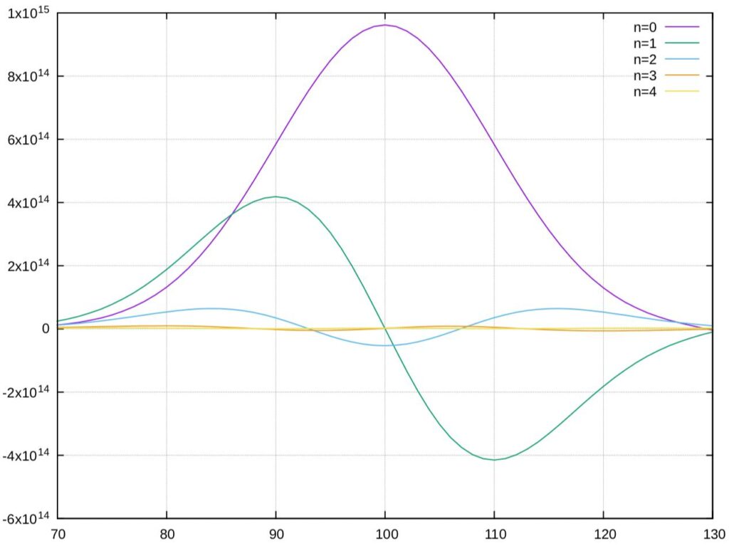
The particular problem we had to solve was to find the energy values for the first 4 energy levels of the potential \( V(x) = x^2/2 \). The approach here is simply to solve our discretised IVP with some estimated energy bounds \(E_{\text{min}}, E_{\text{max}} \), then use the bisection method (yes, the root finding one) to obtain the correct energy for the desired energy level \( N \). You might be wondering how the bisection method can be used; after all, where are the roots? The roots actually correspond to nodes of the wavefunction; the energy estimates are changed based on whether there are too many or too little nodes in the solution. For more on this approach, consider Computational Quantum Mechanics (Izaac & Wang, 2019).
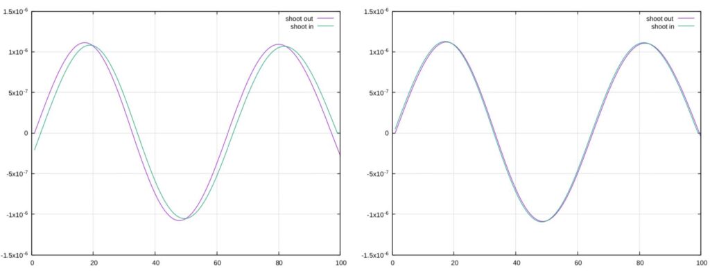
The key drawback of the shooting method is its numerical instability, particularly on the other side of the boundary (i.e the boundary we are iterating towards). To account for this, we can shoot from both ends (so-called forward and backward shooting, or inward and outward shooting depending on the side of reference) and attempt to join the two solutions somewhere in the middle. Although it is possible, it is cumbersome, and there exists other more accurate methods of obtaining a complete solution. To do so, we first make use of a higher-order method to solve the TISE, and then apply a correction formula to synchronise the two solutions. This is the essence of the Numerov-Cooley method.
Numerov-Cooley Method
Numerov’s method is a general method used to solve ODEs of the form \[ y^{\prime\prime}(x) + P(x)y(x) = R(x) \] With some gentle rearranging, the TISE can be written in this form \[ \psi^{\prime\prime}(x)- \frac{2m}{\hbar^2}\left[ V(x) + E \right]\psi(x) = 0 \] As with the shooting method, we must discretise the problem. Instead of merely applying the central difference formula, we can instead use a Taylor series for \( \psi(x + \Delta x) \) and \( \psi(x – \Delta x) \). Adding these two gives us \[ \psi_{n+1} + \psi_{n-1} = 2\psi_n + \psi^{\prime\prime}(x)(\Delta x^2) + \frac{1}{12} \psi^{(4)}(x) (\Delta x^4) + O(\Delta x^6) \] where we have used the shorthand \( \psi_{\pm n}(x) = \psi(x + \pm \Delta x) \) and \( \psi^{(n)} (x) \) to denote the nth derivative of \( \psi(x) \). To deal with the \( \psi^{(4)}(x) \) term, we use the central difference formula (like we did with the shooting method). \[ \psi^{(4)}(x) = \frac{d^2}{dx^2} \psi^{\prime\prime}(x) = \frac{\psi^{\prime\prime}(x+\Delta x)-2\psi^{\prime\prime}(x) + \psi^{\prime\prime}(x-\Delta x)}{(\Delta x)^2} \] and, since we know that \( \psi^{\prime\prime}(x) = -P(x)\psi(x) \) (from the general form of the ODE), we eventually arrive at the following by substitution: \[ \boxed{\psi_{n+1} \left(1 + \frac{(\Delta x)^2}{12}P_{n+1} \right) = 2\psi_n \left(1-\frac{5(\Delta x)^2}{12}P_n \right)- \psi_{n-1} \left( 1 + \frac{(\Delta x)^2}{12}P_{n-1} \right)} \] Now we use this to shoot backwards and forwards with a shooting parameter \( s \ll 1 \).
Suppose we want to use this method to estimate the energy eigenvalues. We could just use a bisection method (as with the normal shooting method), but we can instead make use of a more accurate energy correction known as Cooley’s correction formula. Here the change in energy \( \Delta E \) is given by \[ \Delta E \approx \frac{\psi_m}{\sum_{j=0}^{N-1} |\psi_j |^2} \left[ -\frac{\hbar^2}{2m} \frac{Y_{m+1}+Y_{m-1}-2Y_m}{(\Delta x)^2} + (V_m – E)\psi_m \right] \] where \( Y_m = \left(1 + (\Delta x)^2P_m/12 \right)\psi_m \) and m is the matching point (i.e the point where both the forward and backward shooting solutions meet).
These two methods combined (both the numerical solver and the energy correction) offer a powerful method to estimate energy eigenvalues for arbitrary potentials \( V(x) \).
Direct-Matrix Method
So far we have relied on using discretised equation solvers and energy bisection in order to solve for the energy eigenvalues of some potential \( V(x) \). The direct-matrix method is, as the name implies, a method of directly obtaining the eigenvalues from the TISE in matrix form. To write the TISE in an equivalent matrix form, consider the central difference approximation from the shooting matrix: \[ -\frac{\hbar^2}{2m} \frac{\psi_{j+1}-2\psi_j+\psi_{j-1}}{(\Delta x)^2} + V_j\psi_j = E\psi_j \quad j=1,2,\ldots,N-2\] Let’s introduce the new term \( k = \hbar^2 / (2m\Delta x^2) \) and rewrite the above equation as follows: \[ -k\psi_{j+1} + (2k + V_j)\psi_j-k\psi_{j-1} = E\psi_j \] Now we can write this as a set of coupled linear equations \begin{align*} -k\psi_2 + (2k + V_1)\psi_1 – k\alpha &= E\psi_1 \\
-k\psi_3 + (2k + V_2)\psi_2 – k\psi_1 &= E\psi_2 \\
\vdots & \\
-k\beta + (2k + V_{N-2})\psi_{N-2} – k\psi_{N-3} &= E\psi_{N-2} \end{align*} where we have explicitly included the boundary conditions \( \psi_0 = \alpha \) and \( \psi_{N-1} = \beta \). This is equivalent to the following matrix equation: \begin{equation}
\begin{bmatrix} 2k + V_1 & -k & 0 & \ldots & 0 \\
-k & 2k + V_2 & -k & \ddots & \vdots \\
0 & -k & 2k + V_3 & \ddots & 0 \\
\vdots & \ddots & \ddots & \ddots & -k \\
0 & \ldots & 0 & -k & 2k + V_{N-2} \end{bmatrix} \
\begin{bmatrix} \psi_1 \\ \psi_2 \\ \psi_3 \\ \vdots \\ \psi_{N-2} \end{bmatrix} =
E\begin{bmatrix} \psi_1 \\ \psi_2 \\ \psi_3 \\ \vdots \\ \psi_{N-2} \end{bmatrix} +
k\begin{bmatrix} \alpha \\ 0 \\ \vdots \\ 0 \\ \beta \end{bmatrix}
\end{equation} which can be written more compactly as \( H\mathbf{\psi} = E\mathbf{\psi} + k\mathbf{b} \) where H is the (discretised) Hamiltonian matrix and both \( \mathbf{\psi} \) and \( \mathbf{b} \) are vectors. The solution is thus \[ \psi = k (H-EI)^{-1} \mathbf{b} \] where \( H – EI \) is a symmetric tridiagonal matrix. This can be solved with tridiagonal solver routines in numerical packages such LAPACK or OpenBLAS (assuming you’re using Fortran), or even scipy (for Python). We still need to iterate through values of E in order to find a differentiable solution.
References
- SHPC4001 notes on Computational Quantum Mechanics (now part of the published textbook of the same name by Izaac & Wang, 2019).